Advent of Code 2021
It’s that time of year again. And not just for Secret Santa—it’s time for the Advent of Code, a series of programming puzzles in the lead-up to Christmas.
I’m doing the 2021 challenge in R—in the form of an open-source R package, to demonstrate a test-driven workflow.
Each puzzle description typically comes with a few simple examples of inputs and outputs. We can use these to define expectations for unit tests with the testthat package. Once a function passes the unit tests, it should be ready to try with the main puzzle input.
Check my adventofcode2021 repository on GitHub for the latest.
remotes::install_github('Selbosh/adventofcode2021')- Sonar Sweep
- Dive!
- Binary Diagnostic
- Giant Squid
- Hydrothermal Venture
- Lanternfish
- The Treachery of Whales
- Seven Segment Search
- Smoke Basin
- Syntax Scoring
- Dumbo Octopus
- Passage Pathing
- Transparent Origami
- Extended Polymerization
- Chiton
- Packet Decoder
- Trick Shot
- Snailfish
- Beacon Scanner
- Trench Map
- Dirac Dice
- Reactor Reboot
- Amphipod
- Arithmetic Logic Unit
- Sea Cucumber
Day 1 - Sonar Sweep
Increases
To count the number of times elements are increasing in a vector it’s as simple as
depths <- c(199, 200, 208, 210, 200, 207, 240, 269, 260, 263)
sum(diff(depths) > 0)
## [1] 7for which I defined a function called increases.
Rolling sum
For part two, we first want to calculate the three-depth moving sum, then we count the increases as in part one.
There are plenty of solutions in external R packages for getting lagged (and leading) vectors, for instance dplyr::lag() and dplyr::lead():
depths + dplyr::lead(depths) + dplyr::lead(depths, 2)## [1] 607 618 618 617 647 716 769 792 NA NAOr you could even calculate the rolling sum using a pre-made solution in zoo (Z’s Ordered Observations, a time-series analysis package).
zoo::rollsum(depths, 3)## [1] 607 618 618 617 647 716 769 792To avoid loading any external packages at this stage, I defined my own base R function called rolling_sum(), which uses tail and head with negative lengths to omit the first and last elements of the vector:
head(depths, -2) + head(tail(depths, -1), -1) + tail(depths, -2)## [1] 607 618 618 617 647 716 769 792As David Schoch points out, you can just use the lag argument of diff to make this entire puzzle into a one-liner:
sapply(c(1, 3), \(lag) sum(diff(depths, lag) > 0))## [1] 7 5Day 2 - Dive!
Depth sum
Read in the input as a two-column data frame using read.table().
I gave mine nice column names, cmd and value, but this isn’t essential.
Then take advantage of the fact that TRUE == 1 and FALSE == 0 to make a mathematical ifelse-type statement for the horizontal and vertical movements.
In my R package, this is implemented as a function called dive():
x <- (cmd == 'forward') * value
y <- ((cmd == 'down') - (cmd == 'up')) * value
sum(x) * sum(y)
Cumulative depth sum
Part two is much like part one, but now y represents (change in) aim, and (change in) depth is derived from that.
Don’t forget the function cumsum(), which can save you writing a loop!
Here is the body of my function dive2():
x <- (cmd == 'forward') * value
y <- ((cmd == 'down') - (cmd == 'up')) * value
depth <- cumsum(y) * x
sum(x) * sum(depth)
Day 3 - Binary Diagnostic
Power consumption
There are a few different ways you could approach part one, but my approach was first to read in the data as a data frame of binary integers using the function read.fwf().
Then, find the most common value in each column using the base function colMeans() and rounding the result.
According to the instructions, in the event of a tie you should take 1 to be the most common digit.
Although this is familiar to real life—0.5 rounds up to 1—computers don’t work this way: R rounds to even instead (see ?round).
Because zero is even, that means round(0.5) yields 0.
To get around this, add 1 before rounding, then subtract it again.
My function power_consumption(), which once again takes advantage of TRUE being equivalent to 1 and FALSE to 0:
common <- round(colMeans(x) + 1) - 1
binary_to_int(common) * binary_to_int(!common)
To convert a vector of binary digits to decimal, I use the following utility function:
binary_to_int <- function(x) {
  sum(x * 2 ^ rev(seq_along(x) - 1))
}
However, if using a string representation then there’s a handy function in base R called strtoi() that you could also use for this (thanks to Riinu Pius for that tip).
Life support
Part two finds the common digits in a successively decreasing set of binary numbers. A loop is appropriate here, since we can halt once there is only one number left. As this loop will only run (at most) 12 times in total, it shouldn’t be too slow in R.
Function life_support():
life_support <- function(x) {
  oxygen <- co2 <- x
  for (j in 1:ncol(x)) {
    if (nrow(oxygen) > 1) {
      common <- most_common(oxygen)
      oxygen <- oxygen[oxygen[, j] == common[j], ]
    }
    if (nrow(co2) > 1) {
      common <- most_common(co2)
      co2 <- co2[co2[, j] != common[j], ]
    }
  }
  binary_to_int(oxygen) * binary_to_int(co2)
}
There might be cleverer ways of doing this.
Day 4 - Giant Squid
Bingo
This is one of those problems where half the battle is working out which data structure to use.
I wrote a function read_draws() that reads in the first line of the file to get the drawn numbers, then separately reads in the remainder of the file to get the bingo cards stacked as a data frame.
Later we take advantage of the fact that the bingo cards are square to split the data frame into a list of matrices.
read_draws <- function(file) {
  draws <- scan(file, sep = ',', nlines = 1, quiet = TRUE)
  cards <- read.table(file, skip = 1)
  list(draws = draws, cards = cards)
}
As numbers are called out, I replace them in the dataset with NAs.
Then the helper score_card() counts the number of NAs in each row and column.
If there are not enough, we return zero, else we calculate the score.
score_card <- function(mat, draw) {
  marked <- is.na(mat)
  if (all(c(rowMeans(marked), colMeans(marked)) != 1))
    return(0)
  sum(mat, na.rm = TRUE) * draw
}
Then we put it all together, looping through the draws, replacing numbers with NA and halting as soon as someone wins.
Function play_bingo() is defined as follows, using just base R commands:
play_bingo <- function(draws, cards) {
  size <- ncol(cards)
  ncards <- nrow(cards) / size
  ids <- rep(1:ncards, each = size)

  for (d in draws) {
    cards[cards == d] <- NA
    score <- sapply(split(cards, ids), score_card, draw = d)
    if (any(score > 0))
      return(score[score > 0])
  }
}
Last caller
Part two is very similar, but we throw away each winning bingo card as we go to avoid redundant computation, eventually returning the score when there is only one left.
Here is function play_bingo2(), which uses the same two utility functions:
play_bingo2 <- function(draws, cards) {
  size <- ncol(cards)

  for (d in draws) {
    ncards <- nrow(cards) / size
    ids <- rep(1:ncards, each = size)
    cards[cards == d] <- NA
    score <- sapply(split(cards, ids), score_card, draw = d)
    if (any(score > 0)) {
      if (ncards == 1)
        return(score[score > 0])
      cards <- cards[ids %in% which(score == 0), ]
    }
  }
}
Further optimizations are possible. For example: as written, we calculate every intermediate winner’s score, but we only really need to do it for the first (part 1) and last (part 2) winners.
Also, we could draw more than one number at a time, as we know that nobody’s going to win until at least the fifth draw (for 5×5 cards) and from there, increment according to the minimum number of unmarked numbers on any row or column.
I didn’t bother implementing either of these, as it already runs quickly enough.
Day 5 - Hydrothermal Venture
For a while I tried to think about clever mathematical ways to solve the system of inequalities, but this gets complicated when working on a grid, and where some segments are collinear. In the end it worked out quicker to what seems like a ‘brute force’ approach: generate all the points on the line segments and then simply count how many times they appear.
This is a problem that really lends itself to use of tidyr functions like separate() and unnest(), so naturally I made life harder for myself by doing it in base R, instead.
First, read in the coordinates as a data frame with four columns, x1, y1, x2 and y2.
The nice way to do this is with tidyr::separate() but strsplit() works just fine too.
Here is my parsing function, read_segments():
read_segments <- function(x) {
  lines <- do.call(rbind, strsplit(readLines(x), '( -> |,)'))
  storage.mode(lines) <- 'numeric'
  colnames(lines) <- c('x1', 'y1', 'x2', 'y2')
  as.data.frame(lines)
}
This is one of the few puzzles where the solution to part two is essentially contained in part one.
Depending on how you implement your home-rolled unnest-like function, it could just be a case of filtering out the diagonal lines in part one.
I make liberal use of mapply for looping over two vectors at once.
In the penultimate line, we take advantage of vector broadcasting, which handles all the horizontal and vertical lines where you have multiple coordinates on one axis paired with a single coordinate on the other.
For the diagonal lines, there is a 1:1 relationship so the coordinates just bind together in pairs.
Finally, we work out how to count the rows, without using dplyr::count().
If you convert to a data frame, then table() does this for you.
count_intersections <- function(lines, part2 = FALSE) {
  if (!part2)
    lines <- subset(lines, x1 == x2 | y1 == y2)
  x <- mapply(seq, lines$x1, lines$x2)
  y <- mapply(seq, lines$y1, lines$y2)
  xy <- do.call(rbind, mapply(cbind, x, y))
  sum(table(as.data.frame(xy)) > 1)
}
I’m fairly pleased to get the main solution down to essentially four lines of code, though I’m certain that there are more computationally efficient ways of tackling this problem—if you value computer time more than your own time.
For the tidyverse approach, see David Robinson’s solution.
Day 6 - Lanternfish
In this problem, we have many fish with internal timers. As the instructions suggest, we will have exponential growth, so it’s not a good idea to keep track of each individual fish as you’ll soon run out of memory. On the other hand, there are only nine possible states for any given fish to be in: the number of days until they next reproduce. So we can store a vector that simply tallies the number of fish in each state.
On each day, we can shuffle the fish along the vector, decreasing the number of days for each group of fish by 1, and adding new cohorts of fish at day 6, to represent parent fish resetting their timers, and at day 8 to represent the newly hatched lanternfish.
My short function lanternfish():
lanternfish <- function(x, days = 80) {
  fish <- as.double(table(factor(x, levels = 0:8)))
  for (i in 1:days)
    fish <- c(fish[2:7], fish[8] + fish[1], fish[9], fish[1])
  sum(fish)
}
Because R indexes from 1 rather than 0, the element fish[1] represents the number of fish with 0 days left, fish[2] represents the number with 1 day left, and so on.
If you find this confusing, you can index from zero instead, thanks to the new index0 package:
lanternfish0 <- function(x, days = 80) {
  fish <- as.double(table(factor(x, levels = 0:8)))
  for (i in 1:days) {
    fish <- index0::index_from_0(fish)
    fish <- c(fish[1:6], fish[7] + fish[0], fish[8], fish[0])
   }
  sum(fish)
}
There is a slightly different way to perform the updates. David Robinson suggested an approach based on linear algebra. Here we apply the same procedure as above, but via matrix multiplication. It takes about the same time to run.
lanternfish <- function(x, days = 80) {
  fish <- table(factor(x, levels = 0:8))
  mat <- matrix(0, 9, 9)
  mat[cbind(2:9, 1:8)] <- 1 # decrease timer for fish w/ 1-8 days left
  mat[1, c(7, 9)] <- 1      # add 'new' fish with 6 & 8 days left
  for (i in 1:days)
    fish <- fish %*% mat
  sum(fish)
}
Day 6 is another puzzle where the solutions for parts one and two are essentially the same.
The only thing to be careful of on part two is that you don’t run into integer overflow.
If you do, make sure the numbers you’re adding together are of type double.
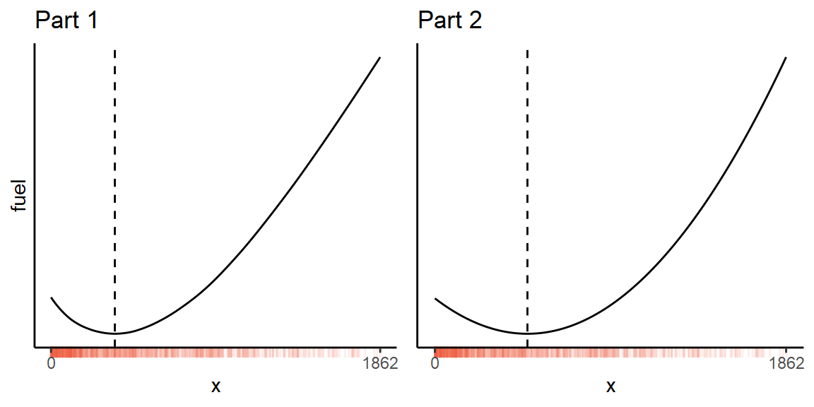
Day 7 - The Treachery of Whales
Median
While it’s possible to brute-force this puzzle by simply calculating the fuel requirement at every single point (within the range of the inputs), you can do it about 200× faster by treating it as an optimization problem.
The total fuel required for any potential position is
x <- scan('input.txt', sep = ',')
f <- function(pos) sum(abs(x - pos))
where x are the initial locations of the crabs.
Then run it through optimize(), and round to the nearest integer position:
sol <- optimize(f, range(x))$minimum
f(round(sol))
However, there is an even faster analytical solution!
sol <- median(x)Thanks to Claire Little for pointing this out.
Mean
Part two just has a slightly different function to optimize. Using the formula for the sum of an arithmetic progression:
f2 <- function(pos) {
  n <- abs(x - pos)
  sum(n / 2 * (1 + n))
}
Then we can simply minimize this function as before.
sol <- optimize(f2, range(x))$minimum
f2(round(sol))
However, there’s a shortcut for this part as well! Calculate the mean of the initial positions, and work out which of the two nearest integers gives the minimum result:
min(
  f2(floor(mean(x))),
  f2(ceiling(mean(x)))
)
Thanks to Jonatan Pallesen. This is about 5 times faster than my optimizer.
And here is what the functions look like for my input dataset:
Day 8 - Seven Segment Search
Unique digits
Read in the data and then the first part is just a one-liner:
input <- do.call(rbind, strsplit(readLines(input_file(8)), '[^a-z]+'))

count_unique <- function(x) {
  sum(nchar(x[, -(1:10)]) %in% c(2, 3, 4, 7))
}
Segment matching
I really wanted to solve part two using graph theory, by representing the puzzle as a maximum bipartite matching problem. However, I couldn’t quite get this to work. My final solution is instead just a lot of leg work.
Essentially you solve the problem by hand and then encode the process programmatically. Recognize that some digits have segments in common, or not in common, and use this to eliminate the possibilities. I stored the solutions in a named vector, which I was able to use to look up the digits found so far.
The function setdiff() comes in useful.
contains <- function(strings, letters) {
  vapply(strsplit(strings, ''),
         function(s) all(strsplit(letters, '')[[1]] %in% s),
         logical(1))
}

output_value <- function(vec) {
  segments <- c('abcefg', 'cf', 'acdeg', 'acdfg', 'bcdf',
                'abdfg', 'abdefg', 'acf', 'abcdefg', 'abcdfg')
  nchars <- setNames(nchar(segments), 0:9)

  # Sort the strings
  vec <- sapply(strsplit(vec, ''), function(d) paste(sort(d), collapse = ''))
  sgn <- head(vec, 10)
  out <- tail(vec, 4)

  # Store the known values
  digits <- setNames(character(10), 0:9)
  unique <- c('1', '4', '7', '8')
  digits[unique] <- sgn[match(nchars[unique], nchar(sgn))]

  # Remaining digits have 5 or 6 segments:
  sgn <- setdiff(sgn, digits)
  digits['3'] <- sgn[nchar(sgn) == 5 & contains(sgn, digits['1'])]
  digits['6'] <- sgn[nchar(sgn) == 6 & !contains(sgn, digits['1'])]
  sgn <- setdiff(sgn, digits)
  digits['0'] <- sgn[nchar(sgn) == 6 & !contains(sgn, digits['4'])]
  sgn <- setdiff(sgn, digits)
  digits['9'] <- sgn[nchar(sgn) == 6]
  sgn <- setdiff(sgn, digits)
  digits['2'] <- sgn[
    contains(sgn, do.call(setdiff,
                          unname(strsplit(digits[c('8', '6')], ''))))
  ]
  digits['5'] <- setdiff(sgn, digits)

  # Combine four output digits:
  as.numeric(paste(match(out, digits) - 1, collapse = ''))
}
Day 9 - Smoke Basin
Lowest points
You can find all the lowest points with a one-liner:
lowest <- function(h) {
  h < cbind(h, Inf)[, -1] &          # right
    h < rbind(h, Inf)[-1, ] &        # down
    h < cbind(Inf, h[, -ncol(h)]) &  # left
    h < rbind(Inf, h[-nrow(h), ])    # up
}
Then do sum(h[lowest(h)]) to get the result, where h is a numeric matrix of the input data.
Basins
The second part is harder and doesn’t immediately lead from the first.
Initially I thought of replacing each lowest point with Inf, then finding the new lowest points and repeating the process until all the basins are found.
However, the basins are simply all points where the height is < 9, so you can find the basins in a single step.
The tricky part is labelling them separately, so you can count up their respective sizes.
The boring way of doing this is just to loop over the indices and label the points that neighbour already-labelled ones (starting with the lowest points as the initial labels), doing several passes until everything (except the 9s) is labelled.
basins <- function(h) {
  l <- lowest(h)
  h[] <- ifelse(h < 9, NA, Inf)
  h[l] <- 1:sum(l)
  while (anyNA(h)) {
    for (i in 1:nrow(h)) for (j in 1:ncol(h)) {
      if (is.na(h[i, j])) {
        nbrs <- h[cbind(c(max(i - 1, 1), min(i + 1, nrow(h)), i, i),
                        c(j, j, max(j - 1, 1), min(j + 1, ncol(h))))]
        if (any(is.finite(nbrs)))
          h[i, j] <- nbrs[is.finite(nbrs)][1]
      }
    }
  }
  sizes <- table(h[is.finite(h)])
  head(sort(sizes, decreasing = TRUE), 3)
}
To vectorize this in the same way as part one, we define a new binary (infix) operator %c%, analogous to dplyr::coalesce().
What this does is replace an NA value (a basin not yet assigned a label) with its finite neighbour, while leaving Infs (marking basin edges) alone.
"%c%" <- function(x, y) {
  ifelse(is.infinite(x), x,
         ifelse(!is.na(x), x,
                ifelse(!is.infinite(y), y, x)))
}
Then the new function for part two is as follows. It is five times faster to run than the nested loop above.
basins2 <- function(h) {
  l <- lowest(h)
  h[] <- ifelse(h < 9, NA, Inf)
  h[l] <- 1:sum(l)
  while(anyNA(h)) {
    h <- h %c%
      cbind(h, NA)[, -1] %c%        # right
      rbind(h, NA)[-1, ] %c%        # down
      cbind(NA, h[, -ncol(h)]) %c%  # left
      rbind(NA, h[-nrow(h), ])      # up
  }
  sizes <- table(h[is.finite(h)])
  head(sort(sizes, decreasing = TRUE), 3)
}
You can also formulate this as an image analysis problem, effectively treating each basin as an area of similar colour to select, or you can treat it as a network theory problem and apply the igraph package to find graph components.
Day 10 - Syntax Scoring
Corrupt characters
Whilst it’s probably possible to do the first part with some very fancy recursive regular expressions, I don’t know how to use them.
Instead, my method of finding unmatched brackets is simply to search for empty pairs of brackets and successively strip them from the string.
Keep doing this until the strings stop changing.
Then, get the first closing bracket (if any), using regmatches().
These are the illegal characters.
My function syntax_score() is implemented as follows:
lines <- readLines('input.txt')
old <- ''
while (!identical(old, lines -> old))
  lines <- gsub(r'(\(\)|<>|\{\}|\[\])', '', lines)
illegals <- regmatches(lines, regexpr(r'(\)|>|\}|\])', lines))
The syntax score is calculated using a named vector as a lookup table.
illegal_score <- c(')' = 3, ']' = 57, '}' = 1197, '>' = 25137)
sum(illegal_score[illegals])
Autocomplete
Part two starts the same, but instead of extracting the illegal characters we just throw away those lines that contain them.
illegals <- grep(r'(\)|>|\}|\])', lines)
chars <- strsplit(lines[-illegals], '')
From here, we can calculate the scores using a Reduce operation (from right to left) with another lookup table.
The final answer is the median score.
complete_score <- c('(' = 1, '[' = 2, '{' = 3, '<' = 4)
scores <- sapply(chars, Reduce, init = 0, right = TRUE,
                 f = \(c, s) 5 * s + complete_score[c])
median(scores)
The function autocomplete() wraps it all together.
Day 11 - Dumbo Octopus
Convoluted octopuses
The process of updating the energy levels can be described using a convolution matrix.
It’s easy—like on Day 11 last year—to use a ready-made solution from an image analysis package for this, namely OpenImageR::convolution().
The convolution matrix, or kernel is \[\begin{bmatrix}1 & 1 & 1 \\1 & 0 & 1 \\1 & 1 & 1\end{bmatrix},\] to be applied on an indicator matrix of ‘flashing’ octopuses, and then added to the result. In R,
kernel <- matrix(1:9 != 5, 3, 3)So we define a function, step1(), that applies a single step of the energy level updating process.
Since each octopus can only flash once in a given step, we keep track of those that have already flashed, as well as those currently flashing.
A short while() loop repeats until no more octopuses flash.
step1 <- function(x) {
  x <- x + 1
  flashing <- flashed <- x == 10
  while (any(flashing)) {
    x <- x + OpenImageR::convolution(flashing, kernel)
    flashing <- x > 9 & !flashed
    flashed <- flashing | flashed
  }
  x[x > 9] <- 0
  x
}
However, there is a base R alternative to OpenImageR::convolution() that you can substitute in, for negligible speed penalty (despite that package being written in C).
add_neighbours <- function(x) {
  I <- nrow(x)
  J <- ncol(x)
  cbind(x[, -1], 0) +  # Right
  rbind(x[-1, ], 0) +  # Down
  cbind(0, x[, -J]) +  # Left
  rbind(0, x[-I, ]) +  # Up
  rbind(cbind(x[-1, -1], 0), 0) + # SE
  rbind(0, cbind(x[-I, -1], 0)) + # NE
  rbind(cbind(0, x[-1, -J]), 0) + # SW
  rbind(0, cbind(0, x[-I, -J]))   # NW
}
Counting flashes
We then solve both parts one and two with a single function that repeatedly applies the updating step and counts the flashes (number of zeros) each time.
By default, it simply completes iter steps and then returns cumulative total number of flashes.
In part2 mode, the function will terminate early if it encounters a step where all the octopuses are flashing and return the iteration number, otherwise it will generate a warning.
count_flashes <- function(x, iter = 100, part2 = FALSE) {
  count <- 0
  for (i in 1:iter) {
    x <- step1(x)
    nflashes <- sum(x == 0)
    if (part2 & nflashes == prod(dim(x)))
      return(i)
    count <- count + nflashes
  }
  if (part2)
    warning('No synchronization detected in ', iter, ' steps')
  count
}
The whole thing runs in about 20 milliseconds on my input dataset, or 60 milliseconds using the base R convolution function.
Day 12 - Passage Pathing
Counting paths
Today’s puzzle is very obviously a graph theory problem, so it would seem intuitive to break out igraph for this. However, the functions in that package are mainly designed for finding the shortest paths from A to B, not a complete list of all possible paths.
Therefore, it’s easier (as far as I can tell) to solve this with your own data structure and a recursive function or two.
Antoine Fabri suggested a rather neat solution of describing the graph with a named list, where the names of the elements describe a node, and the vector contained therein list the other nodes reachable from that point.
We can read in the data as follows:
read_edges <- function(file) {
  edges <- read.table(file, sep = '-', col.names = c('from', 'to'))
  edges <- rbind(edges, setNames(edges, rev(colnames(edges))))
  edges <- edges[edges$to != 'start', ]
  split(edges$to, edges$from)
}
Then we solve part one with a recursive function that, starting from start, traverses a path all the way to end and increments a counter.
To avoid revisiting small caves, we discard any edges to vertices with lowercase names, with the aid of tolower().
count_paths <- function(edgelist, node = 'start') {
  if (node == 'end')
    return(1)
  if (!length(edgelist[[node]]))
    return(0)
  if (node == tolower(node))
    edgelist <- lapply(edgelist, \(v) v[node != v])
  sum(vapply(edgelist[[node]], count_paths, e = edgelist,
             FUN.VALUE = numeric(1)))
}
Revisiting caves
Part two is just a slight adaptation. This time we can’t simply delete small caves as soon as we visit them, so we need to keep track of those visited so far, while keeping the graph intact. Once we find ourselves on a node that we have already visited, it means we are visiting it for the second time, so at this point we can delete all the visited nodes and switch over to the function from part one.
count_paths2 <- function(edgelist, node = 'start', visited = NULL) {
  if (node == 'end')
    return(1)
  if (node == tolower(node)) {
    if (node %in% visited) {
      edgelist <- lapply(edgelist, \(v) v[!v %in% visited])
      return(count_paths(edgelist, node))
    }
    visited <- union(visited, node)
  }
  if (!length(edgelist[[node]]))
    return(0)
  sum(vapply(edgelist[[node]], count_paths2, e = edgelist, visited,
             FUN.VALUE = numeric(1)))
}
R is quite slow at recursion, so this second function takes about 6 seconds to run on my full input data. It may be possible to optimize this further, but that might require the use of igraph, which is written in C, rather than a base R solution.
Day 13 - Transparent Origami
Folding paper
The hardest bit about this puzzle is reading in the data, since we have two different data structures in the same file.
The neatest way of doing this is to find the separator (a blank line) in the middle of the file, then read through the parts of the file before and after this separately. Since there’s only one file to read, you could of course just inspect it in a text editor and find out this line number by hand. But here’s a programmatic method.
n <- which(readLines('input.txt') == '')
paper <- read.table('input.txt', sep = ',', nrows = n - 1,
                    col.names = c('x', 'y'))
folds <- read.table('input.txt', sep = '=', skip = n)
Next, we need a function that’ll fold the paper in half once.
My initial solution, which works perfectly well, is to convert the x and y coordinates to a matrix representation, then simply update the matrix using subset operations.
mat <- with(paper, matrix(0, max(x) + 1, max(y) + 1))
mat[data.matrix(paper) + 1] <- 1
Watch out for R’s one-based indexing.
We want to fold along the coordinate f, which is at index f + 1, and so the indices either side are f and f + 2.
fold_once <- function(x, dir, f) {
  if (dir == 'fold along y') {
    x[, 1:f] | x[, ncol(x):(f + 2)]
  } else {
    x[1:f, ] | x[nrow(x):(f + 2), ]
  }
}
At this point you might notice that the paper is always being folded exactly in half every time.
So the value after the = in the input is actually redundant; it’s always the middle of the matrix.
For instance, in the example data, the matrix has dimension 15×11 and we fold along \(y=7\) (i.e. index 8), which is half of 15.
The next instruction \(x=5\) (index 6) is half of the other dimension.
From here, loop over the directions and then plot the final matrix using image().
Tidy origami
Why do they give us the values to fold along if it’s always the middle value?
Because it’s not actually very efficient to store these sparse coordinates in a matrix.
Instead, recognize, as pointed out by Riinu Pius and Antoine Fabri, that you can just keep the coordinates in a long format and fold them as follows:
fold_once <- function(x, d, f) {
  x[, d] <- ifelse(x[, d] >= f, 2 * f - x[, d], x[, d])
  x[!duplicated(x), ]
}
Then loop over all the instructions with:
fold_paper <- function(x, folds, n = nrow(folds)) {
  for (i in 1:n)
    x <- fold_once(x, folds[i, 1], folds[i, 2])
  x
}
And finally you can plot the result using ggplot2.
library(adventofcode2021)
input <- read_origami(input_file(13))
input$n <- nrow(input[[2]])
folded <- do.call(fold_paper, input)

library(ggplot2)
ggplot(folded) +
  aes(x, y) +
  geom_tile(fill = '#f5c966') +
  coord_fixed() +
  scale_y_reverse() +
  theme_void()
Day 14 - Extended Polymerization
Inserting letters
The initial approach to this problem is to perform the insertions and build up an ever-lengthening string. There might be a way to do this using regular expressions, but I used an approach based on table joins.
First, read in the data:
template <- strsplit(readLines('input.txt', n = 1), '')[[1]]
template <- data.frame(first = head(template, -1),
                       second = tail(template, -1))
rules <- read.table('input.txt', skip = 1)
rules <- data.frame(first  = substr(rules[, 1], 1, 1),
                    second = substr(rules[, 1], 2, 2),
                    insert = rules[, 3])
This should give you two data frames that look something like this:
  first second
1     N      N
2     N      C
3     C      B

   first second insert
1      C      H      B
2      H      H      N
3      C      B      H
4      N      H      C
5      H      B      C
6      H      C      B
7      H      N      C
8      N      N      C
9      B      H      H
10     N      C      B
11     N      B      B
12     B      N      B
13     B      B      N
14     B      C      B
15     C      C      N
16     C      N      C
From here, the method is straightforward.
Join the template with the rules and produce a new template comprised of the pairs first -> insert and insert -> second.
template <- with(merge(template, rules),
                 data.frame(first = c(first, insert),
                            second = c(insert, second)))
Repeat this process the required number of times and we will have a data frame containing all the pairs of letters.
There’s a problem, though: merge() does not preserve row order, so we’ve lost track of which letters are the first and the last in the sequence.
This means counting up the letters in either column first or second is going to undercount by 1.
We could just refer back to the original input, since the first and last letters won’t change.
However, there’s another neat solution, which takes advantage of the fact that all the middle characters will appear in both columns, but the first and last values, if different, will appear an odd number of times.
counts <- (table(unlist(template)) + 1) %/% 2From here, the difference between the minimum and maximum counts is given by:
diff(range(counts))Scalable insertion
The above approach works for part one, but once we increase the iteration count to 40, the data frame or string representation is far too long to store in memory. It simply doesn’t scale.
Rather than keep the entire sequence and then count up the letters at the end, we can instead store pair frequencies.
To do this, we can call dplyr::count() or use a base R approach.
Add a frequency column to the original data frame:
template <- data.frame(first  = head(template, -1),
                       second = tail(template, -1),
                       n = 1)
or if you want to aggregate on initialization, you could use:
template <- as.data.frame(table(template), stringsAsFactors = FALSE)Then after each round of insertions, aggregate() the counts:
data <- with(merge(template, rules),
             data.frame(first = c(first, insert),
                        second = c(insert, second)))
template <- aggregate(n ~ first + second, data, sum)
Finally, the total letter counts are given by:
tab <- xtabs(n ~ first + second, template)
(rowSums(tab) + colSums(tab) + 1) %/% 2
Day 15 - Chiton
The answer is Dijkstra’s algorithm, whether you’re aware of it or not. That is, the problem is a weighted, directed graph and you’ve been tasked with finding the shortest path between two points.
You could write your own implementation in R, but it’ll be slow, so I am going to use the off-the-shelf solution in the igraph package. The hardest task is converting from a matrix into a 2-dimensional lattice graph.
lattice_from_matrix <- function(m) {
  edges <- data.frame(node1 = c(which(row(m) < nrow(m)),
                                which(col(m) < ncol(m))),
                      node2 = c(which(row(m) > 1),
                                which(col(m) > 1)))
  edges <- rbind(edges, setNames(edges, c('node2', 'node1')))
  edges$weight <- m[edges$node2]
  igraph::graph_from_data_frame(edges)
}
Then, just let the algorithm do the work.
lowest_total_risk <- function(g) {
  as.vector(igraph::distances(g, v = 1, to = igraph::vcount(g),
                              mode = 'out', algorithm = 'dijkstra'))
}
For part two, we need to tile the input and then rerun the code again.
tile_matrix <- function(m, times = 5) {
  m <- Reduce(cbind, lapply(seq_len(times) - 1, '+', m))
  m <- Reduce(rbind, lapply(seq_len(times) - 1, '+', m))
  m[m > 9] <- m[m > 9] %% 10 + 1
  m
}
The final search takes about 0.8 seconds, which is faster than any base-R Dijkstra loop would be.
Day 16 - Packet Decoder
Versions
This puzzle takes a long time to read. The solution involves recursive functions that read through the packets and subpackets in turn. My approach takes the bits and throws them away as they are processed, until there are none left (or, for sub-packets, if we have finished parsing the requisite number).
We are working between bases here, so you want a couple of utility functions to convert to and from integers.
to_bits <- function(x) {
  ints <- strtoi(strsplit(x, '')[[1]], 16)
  bits <- sapply(ints, \(n) tail(rev(as.numeric(intToBits(n))), 4))
  as.vector(bits)
}
Unfortunately, strtoi is not your friend for the binary-to-integer conversion, because it will almost surely silently introduce integer overflow on your main input data.
Here’s one I prepared earlier that uses floating point numbers so it won’t overflow.
binary_to_int <- function(x) {
  sum(x * 2 ^ rev(seq_along(x) - 1))
}
Now here’s the main recursion.
packet_versions <- function(bits, depth = 0, rem_subs = Inf, eval = FALSE) {
  acc <- 0
  while (any(bits > 0) & rem_subs > 0) {
    rem_subs <- rem_subs - 1
    version <- binary_to_int(bits[1:3])
    acc <- acc + version
    type <- binary_to_int(bits[4:6])
    bits <- tail(bits, -6)
    if (type == 4) { # literal value
      n_groups <- which.min(bits[seq(1, length(bits), 5)])
      sub <- head(bits, n_groups * 5)
      sub <- sub[(seq_along(sub) - 1) %% 5 > 0]
      # literal_value <- binary_to_int(sub)
      bits <- tail(bits, -n_groups * 5)
      next
    }
    # Operator mode:
    lentype <- bits[1]
    bits <- bits[-1]
    if (lentype == 0) {
      sub_length <- binary_to_int(bits[1:15])
      bits <- tail(bits, -15)
      sub  <- head(bits, sub_length)
      acc <- acc + packet_versions(sub, depth + 1)[['acc']]
      bits <- tail(bits, -sub_length)
    } else {
      n_subs <- binary_to_int(bits[1:11])
      bits <- tail(bits, -11)
      sub_result <- packet_versions(bits, depth + 1, n_subs)
      acc <- acc + sub_result[['acc']]
      bits <- tail(bits, sub_result[['length']])
    }
  }
  if (depth)
    acc <- c(acc = acc, length = length(bits))
  acc
}
Be careful with length type ID 1, because you need to save the number of bits you’ve parsed and then send this number back to the main function. Similarly, it’s a good idea to keep track of how deep in the recursion you are at any given time.
Evaluation
The second part is tricky. I decided to adapt my function from part one to generate syntactically-valid R expressions, so that final step is simply evaluating machine-generated code.
packet_decode <- function(bits, depth = 0, rem_subs = Inf) {
  acc <- NULL
  while (any(bits > 0) & rem_subs > 0) {
    rem_subs <- rem_subs - 1
    type <- binary_to_int(bits[4:6])
    bits <- tail(bits, -6)
    op <- c('sum', 'prod', 'min', 'max', 'c', '`>`', '`<`', '`==`')[type + 1]
    if (type == 4) { # literal value
      n_groups <- which.min(bits[seq(1, length(bits), 5)])
      sub <- head(bits, n_groups * 5)
      sub <- sub[(seq_along(sub) - 1) %% 5 > 0]
      literal_value <- binary_to_int(sub)
      acc$expr <- c(acc$expr, literal_value)
      bits <- tail(bits, -n_groups * 5)
      next
    }
    # Operator mode:
    lentype <- bits[1]
    bits <- bits[-1]
    if (lentype == 0) {
      sub_length <- binary_to_int(bits[1:15])
      bits <- tail(bits, -15)
      sub  <- head(bits, sub_length)
      sub_result <- packet_decode(sub, depth + 1)
      subexpr <- c(op, sub_result[['expr']])
      acc$expr <- c(acc$expr, list(subexpr))
      bits <- tail(bits, -sub_length)
    } else {
      n_subs <- binary_to_int(bits[1:11])
      bits <- tail(bits, -11)
      sub_result <- packet_decode(bits, depth + 1, n_subs)
      subexpr <- c(op, sub_result[['expr']])
      acc$expr <- c(acc$expr, list(subexpr))
      bits <- tail(bits, sub_result[['length']])
    }
  }
  if (depth)
    acc$length <- length(bits)
  acc
}
The structure of the function is essentially the same, and the result is a deeply nested list representing the hierarchical tree of expressions.
From here we want to convert it from a tree into some code, and the function combine_expr does this for us:
combine_expr <- function(node, eval = FALSE) {
  if (length(node) == 1)
    return(node)
  expr <- sprintf('%s(%s)', node[1], paste(node[-1], collapse = ', '))
  if (!eval)
    return(expr)
  eval(str2expression(expr))
}
However, it will only work on leaves of the tree.
How can we correctly operate on the entire tree and turn it into a single expression?
That requires more recursion.
Annoyingly, the function rapply doesn’t quite do what’s needed, so we introduce yet another function, called packet_parse:
packet_parse <- function(tree, eval = FALSE) {
  if (!is.list(tree))
    return(combine_expr(tree, eval))
  expr <- packet_parse(unlist(lapply(tree, packet_parse, eval), use.names = F))
  if (eval & is.character(expr))
    return(eval(parse(text = expr)))
  expr
}
You can choose to view the expression, or evaluate it.
Here is my final expression generated by packet_parse:
sum(prod(425542, `<`(247, 247)), sum(121, 21236), prod(`>`(sum(11, 12, 11), sum(7, 10, 7)), 32566), prod(`<`(sum(8, 7, 15), sum(6, 11, 10)), 4507180), min(prod(prod(sum(prod(max(prod(min(prod(min(prod(max(sum(sum(max(sum(sum(min(prod(prod(130)))))))))))))))))))), 139930778832, prod(`>`(52, 667118), 10), 602147, max(62199), prod(14849899, `<`(11716, 26963)), prod(4083, `>`(135, 135)), prod(135, 217, 224), 73, prod(sum(13, 4, 9), sum(12, 15, 7), sum(13, 10, 9)), min(194), prod(182, 197, 136, 2, 242), prod(226, 142, 34, 124), max(4025, 186042), min(30059, 126119002), min(9, 260, 162), prod(`<`(4, 4), 28699), prod(1945, `==`(1714, 1714)), prod(7, `<`(1545, 108)), sum(12), prod(200, `>`(31050, 655605)), 3154, prod(3, `<`(64896, 116)), 3055, prod(13), min(48082, 226938, 1175, 68077774919), sum(66, 15, 181, 1380642642, 11831587), prod(241, 59), prod(150, `>`(2742, 113)), 37007908601, max(52444, 11, 13008816, 2935), 20723, 8, prod(5, `>`(6241732, 759708)), sum(prod(15, 7, 4), prod(14, 2, 12), prod(13, 6, 6)), sum(2877, 229333, 655820, 1020971), sum(39581, 2, 14), max(982557, 44, 31), 68, prod(`==`(11530, 3492), 41177), prod(`==`(236, 918711093), 3937), max(903466, 228, 6, 25989131, 4028), 229, min(299875, 10969849, 11481, 2281, 13), prod(55300721, `>`(63, 63)), prod(244, `>`(sum(7, 13, 7), sum(12, 5, 14))), prod(4494263, `==`(sum(4, 15, 4), sum(3, 3, 14))), prod(`<`(45, 3307915), 58514), prod(3596530693, `<`(sum(3, 12, 4), sum(9, 11, 2))))Which yields the answer 184487454837 when evaluated.
Day 17 - Trick Shot
A little bit of secondary-school mathematics can help your search for the highest trajectory, and for the total number of trajectories. Key is that the \(x\) and \(y\) movements are essentially independent.
Remember the formula \[ v = u + at \] gives velocity \(v\) at time \(t\) for initial velocity \(u\) and average acceleration \(a\). How long does it take to reach the peak? Rearranging and plugging in values: \[t = \frac{v - u} a = \frac{0 - u}{-1} = u,\] which tells us that the probe launched with vertical velocity \(u\) always reaches its peak at time \(t = u\) (except if pointed downwards: then its highest point is the launch position 0). At that time, the sum of the arithmetic progression is \[ x = \frac{t}2 \Bigl(2u + (t - 1)a\Bigr) = u^2 + \frac{u - u^2}2 = \frac{u(u+1)}{2}, \] for any launch velocity \(u\). Hence, the peak of the curve is always \(\max\{0, u_y(u_y + 1) / 2\}\) where \(u_y\) is the vertical component of \(u\).
Other insights to narrow the search space:
At time \(t\), the probe is at position \[x = \frac{t}2\left(2u - 1+t)\right)\] (using the formula above), so there is no need to loop through successive time points.
Rearrange that formula to get the time it takes for a probe with initial velocity \(u\) to reach point \(x\): \[t = \frac12\left(\sqrt{4u^2+4u-8x+1} + 2u + 1\right).\]
The maximum horizontal velocity \(u_x\) is equal to the right-most edge of the target area. Any faster and the probe will immediately overshoot.
It takes \(t = u_x(u_x+1)/2\) time points for the probe to be slowed down by drag to zero horizontal velocity. This gives us a lower bound \[u_x > \frac12 \left(\sqrt{8x_1+1} - 1\right),\] because if the initial velocity is any less than this then the probe will never reach the left edge of the target area.
In the end I didn’t use all these facts, because a ‘brute force’ type search over several points seems to be fast enough and less fiddly to get the formulae right. But it could certainly be faster if using these points.
search_trajectories <- function(target, trick = TRUE) {
  max_x <- target['x2']
  min_x <- ceiling((sqrt(8 * target['x1'] + 1) - 1) / 2)
  max_y <- -target['y1'] - 1
  min_y <- target['y1']
  n <- 0
  for (y in max_y:min_y) {
    end_time <- time_to_reach(y, target['y1']) - y
    y_seq <- -cumsum(-y:end_time)
    if (min(y_seq) > target['y1'])
      warning('sequence too short for y = ', y)
    for (x in max_x:min_x) {
      x_seq <- cumsum(x:0)
      if (x < end_time + y) {
        x_seq <- c(x_seq, rep(x_seq[x], end_time + y - x))
      } else x_seq <- head(x_seq, end_time + y + 1)
      if (any(x_seq >= target['x1'] & x_seq <= target['x2'] &
              y_seq >= target['y1'] & y_seq <= target['y2'])) {
        if (trick)
          return(y * (y + 1) / 2)
        n <- n + 1
      }
    }
  }
  n
}
In principle—though I couldn’t quite get it to work—we could avoid the loops by calculating the times it takes the probe’s \(y\)-position to reach the top/bottom of the target area, using the time_to_reach formula.
Then plug those times into the position formula to see if the \(x\)-coordinate is also within the target area at those times.
If so, then it hits the target.
position <- function(u, t) {
  t / 2 * (2 * u + (t - 1) * -1)
}

time_to_reach <- function(u, x) {
  round(1/2 * (sqrt(4 * u^2 + 4 * u - 8 * x) + 2 * u + 1))
}
Day 18 - Snailfish
Reduction
I decided (for better or for worse) to convert the square brackets into list(...) expressions, then parse the input as nested lists.
read_sf <- function(input) {
    out <- lapply(input, function(string) {
        expr <- gsub('\\]', ')', gsub('\\[', 'list(', string))
        eval(parse(text = expr))
    })
    if (length(out) == 1) return(unlist(out, FALSE)) else out
}
Then we need to perform the reductions on our list structures.
Splitting is easy, but it’s important that we split only the first node we find and then stop.
I used a counter called done to ensure the rapply loop terminates early.
sf_split <- function(lst) {
    done <- FALSE
    rapply(lst, \(n) {
        if (n <= 9 | done) return(n)
        done <<- TRUE
        list(floor(n / 2), ceiling(n / 2))
    }, how = 'replace')
}
To explode, it’s a bit trickier because you need several nodes to interact with one another.
I wrote some recursive functions to find the depth of the list, to mark the appropriate node with an NA and then to replace it.
I also discovered the relist function, which makes it possible to flatten a list, do some vector operations (handy for getting the indices just before and after our exploded pair) and then return the data to the original nested structure.
depths <- function(lst, depth = 0) {
    if (!is.list(lst)) return(depth)
    unlist(sapply(lst, depths, depth + 1))
}

replaceNA <- function(lst, replacement) {
    if (all(is.na(lst))) return(replacement)
    if (!is.list(lst)) return(lst)
    lapply(lst, replaceNA, replacement)
}

sf_explode <- function(lst) {
    i <- which(depths(lst) > 4)
    L <- i[1]; R <- i[2]
    x <- unlist(lst)
    if (L > 1)
        x[L - 1] <- x[L - 1] + x[L]
    if (R < length(x))
        x[R + 1] <- x[R] + x[R + 1]
    x[c(L, R)] <- NA
    replaceNA(relist(x, lst), 0)
}
Then we put it all together as reduce operations.
sf_reduce <- function(lst) {
    Reduce(\(a, b) list(sf_reduce1(a), b), lst) |> sf_reduce1()
}

sf_reduce1 <- function(lst) {
    if (max(depths(lst)) > 4) lst <- Recall(sf_explode(lst))
    if (any(unlist(lst) > 9)) lst <- Recall(sf_split(lst))
    lst
}
If you try to reduce the whole list in one operation, you’ll definitely get a stack overflow with the larger input datasets. Thus it’s important to reduce from the left until it’s as simple as possible, then combine it with the next line.
My code is quite slow; it might be more sensible to rewrite this as a repeat loop rather than doing all this recursion.
Finally, calculate the magnitude.
magnitude <- function(lst) {
    if (!is.list(lst)) return(lst)
    Reduce(\(a, b) 3 * magnitude(a) + 2 * magnitude(b), lst)
}
Pairs
There might be a clever way of finding the biggest pair but I use brute force:
combos <- t(combn(length(input), 2))
combos <- rbind(combos, combos[, 2:1])
magnitudes <- apply(combos, 1, \(i) magnitude(sf_reduce(input[i])))
max(magnitudes)
Day 19 - Beacon Scanner
Transformers
This was the hardest problem yet. There were a few ideas I had about how to solve the problem quickly, possibly without even having to find any of the actual coordinates. However, I could not work out how to implement them in the end and resorted to the ‘slow’ way: iterating through the scanners one by one and trying the rotations and reflections in turn until they fit into place.
One key insight is that pairwise Euclidean distances within a scanner’s beacons are invariant to translations and rotations. Thus, if we compute within-scanner distance matrix for each one, we know that adjacent scanners must have at least \(12 * (12 - 1) / 2 = 66\) distance pairs in common. This is a good way to set up the initial search strategy.
David Robinson offers a neat solution which finds the rotations and reflections mathematically, rather than by trial and error.
The clever solution, which I suspect I had been looking for but never quite reached, is to think like a statistician should, and find the transformations using linear regression. Thanks to Ryan McCorvie.
Whatever method you go for, read in the data, with judicious handling of NAs to divide up the scanners.
read_scanners <- function(file) {
  input <- read.csv(file, header = FALSE, col.names = c('x', 'y', 'z'))
  input$scanner <- cumsum(is.na(input$z))
  type.convert(na.omit(input), as.is = TRUE)
}
Here is an initial solution, partly inspired by Ashley Baldry. Generate copies of every scanner’s beacons in the various orientations. There are supposed to be 24 different transformations but I ended up with 48.
orientate_scanners <- function(input) {
  mirror <- expand.grid(x = c(1, -1), y = c(1, -1), z = c(1, -1))
  rotate <- expand.grid(x = 1:3, y = 1:3, z = 1:3)
  rotate <- rotate[apply(rotate, 1, \(x) length(unique(x)) == 3), ]
  lapply(split(input, input$scanner), function(s) {
    s <- as.matrix(s)[, 1:3]
    apply(rotate, 1, \(r) s[, r], simplify = F) |>
      lapply(\(m) apply(mirror, 1, \(r) sweep(m, 2, r, '*'), simplify = F)) |>
      unlist(recursive = F, use.names = F)
  })
}
Then loop through the scanners and keep rotating them until the between-scanner distance matrix contains ≥12 common distances, implying that the beacons are in the right orientation and just need translating (by this distance).
locate_scanners <- function(input) {
  scanners <- orientate_scanners(input)
  scanner_coords <- rep(0, 3)
  beacons <- scanners[[1]][[1]]
  scanners <- scanners[-1]
  while (length(scanners)) {
    for (scanner in scanners) {
      done <- FALSE
      for (orientation in scanner) {
        dtbl <- table(dist2(orientation, beacons))
        if (any(dtbl >= 12)) {
          done <- TRUE
          break
        }
      }
      if (!done) next
      scanners <- setdiff(scanners, list(scanner))
      trans <- names(dtbl)[dtbl >= 12]
      trans <- scan(textConnection(trans), quiet = TRUE)
      scanner_coords <- rbind(scanner_coords, trans)
      beacons <- unique(rbind(beacons, sweep(orientation, 2, trans, '+')))
    }
  }
  list(beacons = beacons, scanners = scanner_coords)
}
The helper function dist2 stores the multi-dimensional pairwise distances as a string, and the most common one is then parsed back into a 3-vector using scan.
dist2 <- function(X, Y) {
  apply(X, 1, \(x) apply(Y, 1, \(y) paste(y - x, collapse = ' ')))
}
Linear regression
It’s not particularly satisfactory having a solution that takes over 10 seconds to run for part one, and systematically checking every rotation and reflection seems rather too much like brute force.
The next day, I refactored Ryan McCorvie’s linear regression solution as follows.
read_scanners <- function(file) {
  input <- read.csv(file, header = FALSE, col.names = c('x', 'y', 'z'))
  split(input, cumsum(is.na(input$z))) |>
    lapply('[', -1, ) |>
    lapply(type.convert, as.is = TRUE)
}
scanners <- read_scanners(input_file(19))

# Compute pairwise distances among beacons *within* each scanner.
distances <- lapply(scanners, dist)

# How many such distances does each pair of scanners have in common?
similarity <- combn(distances, 2, \(x) Reduce(intersect, x), simplify = F)

# Using this information, which scanners appear to overlap?
overlaps <- lengths(similarity) >= 12 * (12 - 1) / 2

# Just keep those pairs.
similarity <- similarity[overlaps > 0]

# But it helps if we can remember which they are.
pairs <- t(combn(length(scanners), 2)[, overlaps > 0])

# Match up those beacons that two scanners have in common.
match_beacons <- function(s1, s2) {
  m1 <- as.matrix(distances[[s1]])
  m2 <- as.matrix(distances[[s2]])
  matching <- c()
  for (j1 in 1:ncol(m1)) {
    done <- FALSE
    for (j2 in 1:ncol(m2)) {
      if (length(intersect(m1[, j1], m2[, j2])) >= 12) {
        matching <- rbind(matching, cbind(s1 = j1, s2 = j2))
        done <- TRUE
        break
      }
    }
    if (done) next
  }
  matching
}

# For two scanners, how can we orientate the 2nd to match the 1st?
align_scanners <- function(s1, s2) {
  match <- match_beacons(s1, s2)

  # Time for a bit of linear regression!
  LHS <- scanners[[s1]][match[, 's1'], , drop = F]
  RHS <- scanners[[s2]][match[, 's2'], , drop = F]
  lm_x <- lm(LHS$x ~ x + y + z, RHS)
  lm_y <- lm(LHS$y ~ x + y + z, RHS)
  lm_z <- lm(LHS$z ~ x + y + z, RHS)

  # The predictions gives the beacon coordinates.
  beacon_coords <- as.data.frame(apply(cbind(
    x = predict(lm_x, scanners[[s2]]),
    y = predict(lm_y, scanners[[s2]]),
    z = predict(lm_z, scanners[[s2]])), 2, round))

  # The model intercept is the translation / the scanner position!
  scanner_coords <- apply(cbind(x = coef(lm_x)[1],
                                y = coef(lm_y)[1],
                                z = coef(lm_z)[1]), 2, round)

  # Globally update
  scanners[[s2]] <<- beacon_coords
  beacons <<- unique(rbind(beacons, beacon_coords))
  scanner_locations <<- rbind(scanner_locations, scanner_coords)
}

# Do the search.
found <- 1
to_find <- 2:length(scanners)
scanner_locations <- c(0, 0, 0)
beacons <- scanners[[1]]
while (length(to_find)) {
  overlaps_with_found <- pairs[xor(pairs[, 1] %in% found,
                                   pairs[, 2] %in% found), , drop = F]
  for (i in 1:nrow(overlaps_with_found)) {
    # Let s1 be the already-aligned scanner.
    s1 <- intersect(overlaps_with_found[i, ], found)
    if (length(s1) > 1) next
    s2 <- setdiff(overlaps_with_found[i, ], s1)
    message('Joining ', s1, ' and ', s2)
    align_scanners(s1, s2)
    found <- c(found, s2)
    to_find <- setdiff(to_find, found)
  }
}
As well as being elegant, it’s also far quicker than my initial approach. You can see Ryan’s original code on GitHub.
Manhattan distance
Part two, assuming you’ve been keeping track of the scanner locations or translations, is a one-liner. Distance matrices are a built-in feature of R!
max(dist(result$scanners, 'manhattan'))Day 20 - Trench Map
My test-driven development strategy was caught out here because there are some key qualities of the test dataset that are not found in any of the examples given in the puzzle description.
Eric repeatedly emphasizes that the image space is meant to be infinite, but it’s easy to overlook this and assume it just means the output image will be larger in size than the input image, possibly with coordinate indices below zero.
Firstly, read in the data.
read_pixels <- function(file) {
  input <- readLines(file)
  algorithm <- strsplit(input[1], '')[[1]] == '#'
  img <- do.call(rbind, strsplit(tail(input, -2), '')) == '#'
  list(image = img, algorithm = algorithm)
}
This produces a logical matrix as the input image and a logical vector (of length 512) for the algorithm. Next, we need a way of finding the codes from each pixel’s neighbours. Here is my neat vectorized solution.
binary_neighbours_to_int <- function(x, pad = 0) {
    I <- nrow(x)
    J <- ncol(x)
    . <- pad
    2^8 * rbind(., cbind(., x[-I, -J])) +    # NW
      2^7 * rbind(., x[-I, ]) +              # N
      2^6 * rbind(., cbind(x[-I, -1], .)) +  # NE
      2^5 * cbind(., x[, -J]) +              # W
      2^4 * x +                              # .
      2^3 * cbind(x[, -1], .) +              # E
      2^2 * rbind(cbind(., x[-1, -J]), .) +  # SW
      2^1 * rbind(x[-1, ], .) +              # S
      2^0 * rbind(cbind(x[-1, -1], .), .)    # SE
}
Now we need to run the algorithm itself.
At this point you’ll come up against something that’s easy to overlook: the two end bits of the algorithm.
In the example data, algorithm[1] is equal to zero, so any isolated dark pixels (without any neighbours) that would have a neighbour-sum of zero remain dark.
However, in the test dataset, we have algorithm[1] = 1, which means any empty areas are completely filled (on odd iterations).
Combine this with the fact that algorithm[512] = 0, which switches those pixels off again on every second step.
In fact, it’s not possible for anybody’s puzzle input to have both end bits equal to 1, because then the number of light pixels would be infinite after every single image enhancement step.
How do we use this information? By padding out the image area with the appropriate values—1s or 0s—to model the interaction of the borders of the ‘interesting’ part of the image with the surrounding infinite canvas. There’s no need to count up the pixels we can’t see (since there are infinitely many of them), but we need to anticipate new ones joining the image as it grows.
enhance_image <- function(image, algorithm, n = 1) {
  . <- algorithm[1]
  for (i in 1:n) {
    if (algorithm[1]) . <- !.
    image <- b <- binary_neighbours_to_int(
      cbind(., ., rbind(., ., image, ., .), ., .), pad = .)
    image[] <- algorithm[b + 1]
  }
  image
}
The argument pad (which in the main function is abbreviated to . for readability) alternates between 0 and 1 each step, if (and only if) the first bit of algorithm is equal to 1, which triggers this switching behaviour.
It might seem like a lot of matrix operations but enhance_image() completes all 50 steps in less than 200 milliseconds.
The final answer is just the sum() of the output image.
Day 21 - Dirac Dice
Deterministic dice
For part one, we simply have to play the game.
Just write a while or repeat loop to keep going until someone achieves a score of 1000.
The following code is more verbose than it needs to be:
deterministic_dice <- function(player1, player2) {
  score1 <- score2 <- nrolls <- 0
  dice <- 1:3
  repeat {
    player1 <- (player1 + sum(dice) - 1) %% 10 + 1
    score1 <- score1 + player1
    nrolls <- nrolls + 3
    if (score1 >= 1000) break

    player2 <- (player2 + sum(dice + 3) - 1) %% 10 + 1
    score2 <- score2 + player2
    nrolls <- nrolls + 3
    if (score2 >= 1000) break

    dice <- (dice + 6 - 1) %% 100 + 1
  }
  prod(nrolls, min(score1, score2))
}
Quantum states
Part two calls for recursion, and with some optimization if you want your code to run in any reasonable time frame. This means that at every opportunity, if there is room to ignore or delete universes that are redundant, we should do so.
Each player is still rolling the die three times, but there are only 7 possible unique sums of the values 1, 2 and 3:
rolls <- table(rowSums(expand.grid(1:3, 1:3, 1:3)))
rolls <- mapply(c, sum = as.numeric(names(rolls)), n = rolls, SIMPLIFY = F)
Then, at each set of rolls, we recursively count up the number of wins associated with each player for the sum of those rolls. We only need one function to do this: for player 2’s wins, we can just swap the players and accumulated scores around and pretend that player 2 is now player 1.
dirac_dice <- function(player1, player2) {
  count_wins <- memoise::memoise(
    function(player1, player2, score1, score2) {
      Reduce(
        \(wins, roll) {
          player1 <- (player1 + roll['sum'] - 1) %% 10 + 1
          score1 <- score1 + player1
          if (score1 >= 21) {
            return(wins + c(roll['n'], 0))
          } else
            wins + roll['n'] *
            rev(count_wins(player2, player1, score2, score1))
        },
        rolls,
        init = c(w1 = 0, w2 = 0))
    })
  max(count_wins(player1, player2, 0, 0))
}
To avoid revisiting universes, some caching is useful, so we can look up the value of any function call that has already been made. You could store and look up these results in a named vector, or you could do it the lazy way like I did and use the package memoise, which simply does this for you behind the scenes.
My code takes about two minutes to run for part two. Not quick, but R isn’t very fast at recursive function calls.
Day 22 - Reactor Reboot
On day 22, it’s pretty obvious from the outset that the ‘obvious’ solution to part one—explicitly keeping track of all the cubes—is not going to work at all when the problem scales up for part two.
I won’t even bother to show the ‘slow’ method here, and we can focus on the scalable solution. Rather than look after one row for every cube (or at least every switched-on cube) in the reactor, we need to store the boundaries of the cuboids only, in a similar format to how they are given in the input.
The tricky part here is that the union or difference of two overlapping cuboids (or more generally, 3-dimensional intervals) cannot, in general be described as two cuboids: the new shape is non-convex.
What we need to do is partition the two input cuboids into a several smaller non-overlapping ones, and then do the union operation (making sure not to double-count the intersection) or the set-difference operation (subtracting the intersection from the first cuboid).
For example, consider, in two dimensions, two cuboids A and B:
 ________           ____             ___              ____           ___
| A   __|____      | A1|   ____     |__| } A2        | A1|   ____   |__| A3  ___
|____|__|   |  =   |___|  | B1|  +  |__| } }      =  |___|  | B1|    ___    |__| C
     |____B_|             |___|     |__|   } B2             |___|   |__| B3
I decided to use object-orientated programming for this, through the R6 package.
This allows me to define a new Cuboid class, with fields describing the x, y and z ranges, and to write methods to—if an instance of a cuboid is overlapping with another—divide the two into a set of non-overlapping ones to perform the necessary set operations.
Cuboid <- R6::R6Class('Cuboid',
    public = list(
        x = NULL, y = NULL, z = NULL,
        initialize = function(x, y, z) {
            self$x <- x
            self$y <- y
            self$z <- z
        },
        volume = function() {
            (diff(self$x) + 1) *
            (diff(self$y) + 1) *
            (diff(self$z) + 1)
        },
        cubes = function() { # for debugging purposes
            expand.grid(self$x[1]:self$x[2],
                        self$y[1]:self$y[2],
                        self$z[1]:self$z[2])
        },
        is_overlapping = function(that) {
            is_overlapping(self$x, that$x) &&
            is_overlapping(self$y, that$y) &&
            is_overlapping(self$z, that$z)
        },
        remove = function(that) {
            stopifnot(is.R6(that))
            if (!self$is_overlapping(that))
              return(list(self))
            x <- self$x
            y <- self$y
            z <- self$z
            olx <- interval_intersect(x, that$x)
            oly <- interval_intersect(y, that$y)
            setdiff <- list(
                if (that$x[1] > x[1])
                    Cuboid$new(c(x[1], that$x[1] - 1), y, z),
                if (that$y[1] > y[1])
                    Cuboid$new(olx, c(y[1], that$y[1] - 1), z),
                if (that$y[2] < y[2])
                    Cuboid$new(olx, c(that$y[2] + 1, y[2]), z),
                if (that$z[1] > z[1])
                    Cuboid$new(olx, oly, c(z[1], that$z[1] - 1)),
                if (that$z[2] < z[2])
                    Cuboid$new(olx, oly, c(that$z[2] + 1, z[2])),
                if (that$x[2] < x[2])
                    Cuboid$new(c(that$x[2] + 1, x[2]), y, z)
            )
            setdiff[lengths(setdiff) > 0]
        }
    )
)
We only need a remove() method, because to get the union of two cuboids A and B, we can remove B from A, then add B again and the intersection will only be counted once.
Then our data import functions are:
read_cubes <- function(file) {
    input <- gsub("[xyz]=", "", readLines(file))
    input <- strsplit(input, "[ ,]|\\.{2}")
    out <- type.convert(as.data.frame(do.call(rbind, input)), as.is = TRUE)
    setNames(out, c("mode", "x1", "x2", "y1", "y2", "z1", "z2"))
}

cuboid_list <- function(reactor) {
    # Generate list of R6 'Cuboid' class objects.
    cuboids <- apply(reactor[, -1], 1, \(i)
        list(set = list(Cuboid$new(i[c('x1', 'x2')],
                                   i[c('y1', 'y2')],
                                   i[c('z1', 'z2')]))),
                                   simplify = FALSE)
    # Label with the modes.
    mapply(c, cuboids, reactor$mode, SIMPLIFY = FALSE)
}
And, with the help of a few utilities:
cuboid_setdiff <- function(set, x) {
  unlist(lapply(set, \(y) y$remove(x)))
}

interval_intersect <- function(a, b) {
    c(max(a[1], b[1]), min(a[2], b[2]))
}

is_overlapping <- function(a, b) {
    a[1] <= b[2] && a[2] >= b[1]
}
We can then call our main function:
reboot_reactor <- function(reactor, init = FALSE) {
    if (init)
      reactor <- reactor[abs(reactor$x1) <= 50 &
                         abs(reactor$x2) <= 50, ]
    cuboids <- cuboid_list(reactor)
    rebooted <-
        Reduce(cuboids, f = \(a, b) {
               setdiff <- cuboid_setdiff(a$set, b$set[[1]])
               if (b[[2]] == 'off')
                   return(list(set = setdiff))
               list(set = union(setdiff, b$set))
        })
    sum(sapply(rebooted$set, \(x) x$volume()))
}
This is surprisingly quick, at least by R standards.
Day 23 - Amphipod
Day 23 was where everything went a bit off the rails, because many people in the AoC community were able to solve the puzzle by hand without any coding. However, some starting positions were harder to solve than others, and some people (including me) are simply not very good at puzzles like this.
At that point it’s slightly dispiriting when, if you look online for hints, you don’t find any because everyone just says they solved theirs by hand. It also, arguably, departs from a test-driven development paradigm and the idea that solutions are scalable and applicable to any input dataset.
Long story short: I couldn’t solve mine by hand initially and so had to write some code!
The complete program is quite long as it includes lots of tedious stuff like defining the distances between all the points on the grid and all the pathways along hallways from one amphipod room to another. You can read it in full on GitHub.
As yesterday, I employed R6 classes to store the states, and as on the day before, used a form of caching to get rid of previously-visited or suboptimal states. Specifically, each state describes the positions of all the amphipods, and at each step we explore all the possible states you could go to from here, and their associated costs.
Here is the main loop:
min_amphipod_energy <- function(start) {
  states <- list(start)
  best_score <- Inf
  while (length(states)) {
    new_states <- list()
    for (state in states) {
      if (is.finite(best_score))
        message('Best score: ', best_score)
      for (move in valid_moves(state)) {
        if (move$finished) {
          best_score <- min(best_score, move$score)
        } else if (move$score < best_score) {
          if (move$key %in% names(new_states)) {
            old_score <- new_states[[move$key]]$score
            if (old_score > move$score)
              new_states[[move$key]]$score <- move$score
          } else new_states[[move$key]] <- move
        }
      }
    }
    message('Exploring ', length(new_states), ' new states')
    states <- new_states
  }
  best_score
}
This relies on my custom State class:
State <- R6::R6Class(
  'State',
  public = list(
    rooms = NULL,     # named vector, A1, A2, B1, B2, C1, C2, D1, D2
    hallways = NULL,  # vector of length 7. Unnamed but order is important.
    score = NULL,
    finished = NULL,
    key = NULL,
    initialize = function(rooms, hallways = NULL, score = 0) {
      self$rooms <- rooms
      self$hallways <- if(!is.null(hallways)) hallways else rep('.', 7)
      self$score <- score
      self$finished <- all(self$hallways == '.') &&
        all(self$rooms == rep(LETTERS[1:4], each = length(rooms) / 4))
      self$key = paste(c(hallways, rooms), collapse = ',')
    },
    move = function(from, to, from_hallway, score) {
      rooms <- self$rooms
      hallways <- self$hallways
      if (from_hallway) {
        rooms[to] <- hallways[from]
        hallways[from] <- '.'
      } else {
        hallways[to] <- rooms[from]
        rooms[from] <- '.'
      }
      State$new(rooms, hallways, score)
    })
)
And the bulk of the code is in the method that enumerates all the possible valid moves from any given starting position.
valid_moves <- function(state) {
  room_depth <- length(state$rooms) / 4
  if (room_depth == 4)
    distance <- distance2
  moves <- NULL
  for (i in seq_along(state$hallways)) {
    amphipod <- state$hallways[i]
    # If this spot is empty, nothing to move.
    if (amphipod == '.')
      next
    dest <- paste0(amphipod, seq_len(room_depth))
    # If destination room contains other, different amphipods.
    if (any(setdiff(LETTERS[1:4], amphipod) %in% state$rooms[dest]))
      next
    # If any hallway between here and destination is blocked.
    path <- hallway_paths[[i]][[amphipod]]
    if (any(state$hallways[path] != '.'))
      next
    # Move to the deepest available space in destination room.
    dest <- dest[max(which(state$rooms[dest] == '.'))]
    score <- state$score + distance[i, dest] * move_cost[amphipod]
    moves <- c(moves, state$move(from = i,
                                 to = dest,
                                 from_hallway = TRUE,
                                 score = score))
  }
  for (i in seq_along(state$rooms)) {
    amphipod <- state$rooms[i]
    room_cell <- names(amphipod)
    room <- substring(room_cell, 1, 1)
    pos_in_room <- as.integer(substring(room_cell, 2, 2))
    # If this spot is empty, nothing to move.
    if (amphipod == '.')
      next
    # Can't leave this room if our exit is blocked by another amphipod.
    if (pos_in_room > 1 && state$rooms[i - 1] != '.')
      next
    # No point in leaving destination room except to let other types out.
    if (room == amphipod &&
        all(state$rooms[paste0(room, pos_in_room:room_depth)] == amphipod))
      next
    # Which hallway tile should we move to?
    empty_hallways <- which(state$hallways == '.')
    for (h in empty_hallways) {
      if (all(hallway_paths[[h]][[room]] %in% empty_hallways)) { # not blocked
        score <- state$score + distance[h, room_cell] * move_cost[amphipod]
        moves <- c(moves, state$move(from = i,
                                     to = h,
                                     from_hallway = FALSE,
                                     score = score))
      }
    }
  }
  moves[order(sapply(moves, \(s) s$score))]
}
Final solution runs in about two minutes, for both parts.
The code above works for both, with a slight tweak to the definitions of the starting position and of the distance matrix for part two.
Day 24 - Arithmetic Logic Unit
You can’t brute-force your way out of this one simply by parsing the code into R syntax and evaluating it for all the \(9^{14}\) different input permutations.
This was another puzzle I didn’t really like, because you can’t solve it through test-driven development (except to check the validity of your final answer).
Essentially, the whole puzzle is in the input.txt file rather than the instructions on the web site.
It’s also not immediately obvious what your input dataset has in common with other people’s, so the definition of a ‘general purpose’ solution becomes quite nebulous.
Peek at the input.txt file and work backwards from the bottom.
mul y 0
add y w
add y 5
mul y x
add z y
Here the value +5 on the middle line will probably be different for your input (call it \(\delta y\)), but everything else should be about the same.
For the programme to be valid, the final value assigned to z must be equal to zero.
We have \(z_\text{end} \leftarrow z + y = 0\).
The line mul y 0 resets y to zero (irrespective of its previous value) so the final equation can be rewritten as
\[z + (w + 5)x = 0.\]
Browse through the rest of the programme and you should soon infer the following key points.
- The code is split into 14 chunks of equal length.
- Each starts with
wbeing assigned an input value. - The variable
wis never manipulated apart from this. - The symbols
xandyare auxiliary variables. - The variable
zrepresents a stack, which is “popped” every time we seez div 26and is “pushed” by a value ofyeach time we seeadd z y. Exactly one of these operations happens per chunk.
Now, refer to the equation above.
Since w is equal to an input digit, we have \(1 \leq w \leq 9\), therefore the expression inside the brackets is strictly positive and the equation can only hold when \(x = 0\).
So what is \(x\)? Work a bit further back through the code to the start of chunk 14 and we see:
inp w
mul x 0    # reset memory of x
add x z
mod x 26   # stack.pop()
div z 26
add x -11  # dx <- -11
eql x w    # stack.pop() - 11 == input
eql x 0    # stack.pop() - 11 != input
Remember we need \(x = 0\) at the final line, so the final expression needs to be FALSE.
In other words, the penultimate expression must be TRUE: the top value of the stack, minus 11 (\(\delta x\)), is equal to the most recent input value (w).
\[\text{stack}_1 = w - \delta x\]
So what is the top value of the stack? At the end of the previous (\(i-1\)st) chunk:
mul y 0    # reset memory of y
add y w    # y <- input
add y 8    # input(i-1) + 8
mul y x    # (x is 0 or 1 at this stage)
add z y    # push input(i-1) + 8 onto the stack
The value 8 corresponds to \(\delta y\) but for the previous chunk; let’s call it \(\delta y_{i-1} = 8\). Putting it all together, we get
\[w_{i-1} + \delta y_{i-1} = w_{i} - \delta x_1.\] where \(i\) is the current chunk where the stack is being popped, and \((i-1)\) represents the last time that something was added to the stack (which could be several chunks before).
Our code, then, just has to pick input values that satisfy these pairs of equations, for each pair of chunks, while maximizing or minimizing the 14-digit input number.
read_alu <- function(file) {
    instr <- read.table(file, fill = NA,
                        col.names = c('op', 'lhs', 'val'), row.names = NULL)
    instr$op <- sub('mul', '*', instr$op)
    instr$op <- sub('add', '+', instr$op)
    instr$op <- sub('eql', '==', instr$op)
    instr$op <- sub('div', '%/%', instr$op)
    instr$op <- sub('mod', '%%', instr$op)
    instr$rhs <- ifelse(instr$op == 'inp', '', instr$lhs)
    instr$op <- sub('inp', 'inputs[1]; inputs <- inputs[-1]', instr$op)
    instr$expr <- with(instr, paste(lhs, '<-', rhs, op, val))
    instr$chunk <- cumsum(instr$val == '')
    instr
}

alu_model_number <- function(instructions, minimize = FALSE) {
  digits <- integer(14)
  chunks <- split(instructions, instructions$chunk)
  z_stack <- c()
  for (i in seq_along(chunks)) {
    dx <- as.integer(chunks[[i]]$val[6])  # where x + val
    dy <- as.integer(chunks[[i]]$val[16]) # where y + val (& val != 25)
    pop <- chunks[[i]]$val[5] == 26 # z %% val
    if (!pop) { # 'Push' (append) a value onto the stack.
      z_stack <- c(list(c(dy = dy, pushed = i)), z_stack)
    } else { # 'Pop' (extract) the last value from the stack.
      dy <- z_stack[[1]]['dy']
      pushed <- z_stack[[1]]['pushed']
      z_stack <- z_stack[-1]
      w <- (1:9)[(1:9 + dx + dy) %in% 1:9]
      w <- if (minimize) min(w) else max(w)
      digits[pushed] <- w
      digits[i] <- w + dx + dy
    }
  }
  paste(digits, collapse = '')
}
You can check your working with a unit test that simply evaluates the ALU code with the input values:
alu <- read_alu(input_file(24))
model_number <- alu_model_number(alu)
inputs <- as.numeric(strsplit(model_number, '')[[1]])
w <- x <- y <- z <- 0
eval(str2expression(alu$expr))
expect_equal(z, 0)
Day 25 - Sea Cucumber
We finish on a relatively easy one.
Using a similar style to earlier puzzles, we can find the neighbours in a grid through clever use of rbind() and cbind().
It’s easy to adapt so that one side of the map wraps around to the other.
move_cucumbers <- function(cucumbers) {
  old <- cucumbers
  i <- 0
  repeat {
    new <- move_cucumbers_once(old)
    i <- i + 1
    if (identical(new, old))
      break
    old <- new
  }
  return(i)
}

move_cucumbers_once <- function(x) {
  # First move west to east.
  next_state <- x
  west  <- cbind(x[, ncol(x)], x[, -ncol(x)])
  east  <- cbind(x[, -1], x[, 1])
  # Create an empty spot as cucumbers leave it.
  next_state[x == '>' & east == '.'] <- '.'
  # Occupy the empty spot as cucumbers enter it.
  next_state[x == '.' & west == '>'] <- '>'

  # Now move north to south.
  x <- next_state
  north <- rbind(x[nrow(x), ], x[-nrow(x), ])
  south <- rbind(x[-1, ], x[1, ])
  next_state[x == 'v' & south == '.'] <- '.'
  next_state[x == '.' & north == 'v'] <- 'v'

  return(next_state)
}
There is no part two for day 25: the second star is awarded for completing all of the other stars.