Advent of Code is a series of programming puzzles you can tackle to hone your coding skills each day in the run-up to Christmas.

This year I am attempting it using R, which can make some challenges easier or harder depending on whether they are more ‘computer sciencey’ or more ‘data sciencey’. Generally it makes parsing datasets easier but low-level string manipulation more fiddly.

Here are my solutions so far. Where possible, I’ve tried to strike a balance between efficiency and readability, and to avoid using the packages I might usually use (e.g. dplyr) if I think it makes the puzzle too easy.

The input data are different for each participant, so your numerical results may differ from mine.

1. Report repair
2. Password philosophy
3. Toboggan trajectory
4. Passport processing
5. Binary boarding
6. Custom customs
7. Handy haversacks
8. Handheld halting
9. Encoding error
10. Adapter array
11. Seating system
12. Rain risk
13. Shuttle search
14. Docking data
15. Rambunctious recitation
16. Ticket translation
17. Conway cubes
18. Operation order
19. Monster messages
20. Jurassic jigsaw
21. Allergen assessment
22. Crab combat
23. Crab cups
24. Lobby layout
25. Combo breaker

Day 1 - Report repair

Two numbers

Find the two entries that sum to 2020, then multiply those two numbers together.

This can be a one-liner:

input <- as.integer(readLines('input01.txt'))
prod(input[(2020 - input) %in% input])

[1] 468051

Three numbers

Find the three entries that sum to 2020, then multiply them together.

It might be tempting to go for a naïve solution like this:

prod(combn(input, 3)[, combn(input, 3, sum) == 2020])

[1] 272611658

It gives the right answer but involves a fair amount of unnecessary computation. It takes more than a second to run. If we assume all the inputs are non-negative, we can take advantage of this to reduce the number of operations.

. <- expand.grid(input, input[(2020 - input) > min(input)])
. <- transform(., Var3 = 2020 - Var1 - Var2)
. <- subset(., Var3 > min(input))
prod(.[which.max(.$Var3 %in% input), ])

[1] 272611658

This is approximately 2000 times faster than the one-liner, and works by successively discarding values that could only add up to more than 2020. The . notation is just so I can write this without using dplyr/magrittr.

Day 2 - Password philosophy

Number of letters

How many passwords are valid according to the policies?

1-3 a: abcde
1-3 b: cdefg
2-9 c: ccccccccc

First read in the data. I like data frames and so should you.

input <- readLines('input02.txt')
passwords <- do.call(rbind, strsplit(input, '[- ]|\\: '))
passwords <- setNames(as.data.frame(passwords),
                      c('min', 'max', 'letter', 'password'))
passwords <- transform(passwords,
                       min = as.integer(min),
                       max = as.integer(max))
head(passwords)

  min max letter          password
1  14  15      v  vdvvvvvsvvvvvfpv
2   3  11      k  kkqkkfkkvkgfknkx
3   6  10      j        jjjjjjjjjj
4   5  10      s nskdmzwrmpmhsrzts
5  13  15      v   vvvvvvkvvvvjzvv
6  11  13      h    hhhhhbhhhhdhhh

String operations are a bit of a pain in base R so it’s easier just to use a package, like stringi or stringr for this.

with(passwords, {
     n <- stringr::str_count(password, letter)
     sum(n >= min & n <= max)
})

[1] 625

You could also split each password with strsplit and count the letters with an sapply-type loop.

Position of letters

Now the two digits describe two indices in the password, exactly one of which must match the given letter.

with(passwords,
     sum(xor(substr(password, min, min) == letter,
             substr(password, max, max) == letter))
)

[1] 391

Initially I got caught out here, by misreading the question as ‘at least one’ and then wondering why an inclusive or (|) was returning the incorrect answer.

Day 3 - Toboggan trajectory

The input looks a bit like this:

..##.........##.........##.........##.........##.........##.......  --->
#...#...#..#...#...#..#...#...#..#...#...#..#...#...#..#...#...#..
.#....#..#..#....#..#..#....#..#..#....#..#..#....#..#..#....#..#.
..#.#...#.#..#.#...#.#..#.#...#.#..#.#...#.#..#.#...#.#..#.#...#.#
.#...##..#..#...##..#..#...##..#..#...##..#..#...##..#..#...##..#.
..#.##.......#.##.......#.##.......#.##.......#.##.......#.##.....  --->
.#.#.#....#.#.#.#....#.#.#.#....#.#.#.#....#.#.#.#....#.#.#.#....#
.#........#.#........#.#........#.#........#.#........#.#........#
#.##...#...#.##...#...#.##...#...#.##...#...#.##...#...#.##...#...
#...##....##...##....##...##....##...##....##...##....##...##....#
.#..#...#.#.#..#...#.#.#..#...#.#.#..#...#.#.#..#...#.#.#..#...#.#  --->

Encountering trees

Starting at the top-left corner of your map and following a slope of right 3 and down 1, how many trees would you encounter?

input <- readLines('input03.txt')

A complicated-sounding problem but the solution is mainly mathematical.

positions <- (3 * (seq_along(input) - 1)) %% nchar(input) + 1
sum(substr(input, positions, positions) == '#')

[1] 268

The sequence of positions goes 1, 4, 7, …, and when it reaches the edge of the map, loops back round to the beginning. Using the modulo operator we can use the sequence modulo the width of the input map, then add one because R indexes from one rather than from zero.

Different slopes

Simply wrap the above into a function.

trees <- function(right, down = 1) {
  vertical <- seq(0, length(input) - 1, by = down) + 1
  horizontal <- (right * (seq_along(input) - 1)) %% nchar(input) + 1
  horizontal <- head(horizontal, length(vertical))
  as.double(
    sum(substr(input[vertical], horizontal, horizontal) == '#')
  )
}
trees(1) * trees(3) * trees(5) * trees(7) * trees(1, 2)

[1] 3093068400

The as.double bit is necessary only because multiplying large integer outputs together can cause an overflow when the product is larger than 10⁹.

Day 4 - Passport processing

The example input is in this ragged format, where keys and values are separated by colons and records are separated by double newlines. The first step is to parse this unusual data format.

ecl:gry pid:860033327 eyr:2020 hcl:#fffffd
byr:1937 iyr:2017 cid:147 hgt:183cm

iyr:2013 ecl:amb cid:350 eyr:2023 pid:028048884
hcl:#cfa07d byr:1929

hcl:#ae17e1 iyr:2013
eyr:2024
ecl:brn pid:760753108 byr:1931
hgt:179cm

hcl:#cfa07d eyr:2025 pid:166559648
iyr:2011 ecl:brn hgt:59in

input <- strsplit(readLines('input04.txt'), ' ')
ids = cumsum(!lengths(input))
pairs <- lapply(strsplit(unlist(input), ':'), setNames, c('key', 'value'))
passports <- data.frame(id = rep(ids, lengths(input)),
                        do.call(rbind, pairs))

Missing fields

Now the data are in a standard format, this is a simple split-apply-combine operation. I am using the base aggregate but this could be done equally well using dplyr or data.table.

required <- c('byr', 'iyr', 'eyr', 'hgt', 'hcl', 'ecl', 'pid')
valid <- aggregate(key ~ id, passports,
                   function(x) !length(setdiff(required, x)))
head(valid, 10)

   id   key
1   0  TRUE
2   1  TRUE
3   2  TRUE
4   3  TRUE
5   4  TRUE
6   5  TRUE
7   6  TRUE
8   7 FALSE
9   8 FALSE
10  9  TRUE

Then the answer is simply

sum(valid$key)

[1] 190

Field validation

Thanks to the way we imported the data, this is quite straightforward. The rules are:

• byr (Birth Year) - four digits; at least 1920 and at most 2002.
• iyr (Issue Year) - four digits; at least 2010 and at most 2020.
• eyr (Expiration Year) - four digits; at least 2020 and at most 2030.
• hgt (Height) - a number followed by either cm or in:
  • If cm, the number must be at least 150 and at most 193.
  • If in, the number must be at least 59 and at most 76.
• hcl (Hair Color) - a # followed by exactly six characters 0-9 or a-f.
• ecl (Eye Color) - exactly one of: amb blu brn gry grn hzl oth.
• pid (Passport ID) - a nine-digit number, including leading zeroes.
• cid (Country ID) - ignored, missing or not.

The data are all different types (integer, double and categorical) so the first step will be to spread the table to a wider format, with one row per passport, and one column for each field.

Here is a dplyr + tidyr solution.

library(dplyr)
library(tidyr)
passports_wide <- passports %>%
  pivot_wider(names_from = key, values_from = value) %>%
  mutate(byr = as.integer(byr),
         iyr = as.integer(iyr),
         eyr = as.integer(eyr),
         hgt_value = as.numeric(gsub('cm|in$', '', hgt)),
         hgt_unit = gsub('\\d*', '', hgt))
head(passports_wide)

# A tibble: 6 x 11
     id   iyr cid   pid        eyr hcl     ecl      byr hgt   hgt_value hgt_unit
  <int> <int> <chr> <chr>    <int> <chr>   <chr>  <int> <chr>     <dbl> <chr>   
1     0  1928 150   4761132~  2039 a5ac0f  #25f8~  2027 190         190 ""      
2     1  2013 169   9200769~  2026 #fffffd hzl     1929 168cm       168 "cm"    
3     2  2011 <NA>  3284128~  2023 #6b5442 brn     1948 156cm       156 "cm"    
4     3  2019 279   6749079~  2020 #602927 amb     1950 189cm       189 "cm"    
5     4  2015 <NA>  4736300~  2022 #341e13 hzl     1976 178cm       178 "cm"    
6     5  2020 <NA>  6281139~  2023 #866857 blu     1984 163cm       163 "cm"    

From here, we can filter out the invalid entries, using filter or subset.

passports_wide %>%
  filter(byr >= 1920, byr <= 2002,
         iyr >= 2010, iyr <= 2020,
         eyr >= 2020, eyr <= 2030,
         hgt_value >= 150 & hgt_value <= 193 & hgt_unit == 'cm' |
           hgt_value >= 59 & hgt_value <= 76 & hgt_unit == 'in',
         grepl('^#[0-9a-f]{6}$', hcl),
         ecl %in% c('amb', 'blu', 'brn', 'gry', 'grn', 'hzl', 'oth'),
         grepl('^\\d{9}$', pid)) -> valid_passports
nrow(valid_passports)

[1] 121

You could also use a filtering join, though since most of the fields are ranges of integer values, you would want to use a data.table non-equi-join rather than a simple semi_join.

Day 5 - Binary boarding

Highest seat ID

This task is easy, as soon as you recognise that it is just converting numbers from binary to decimal, where F and L denote ones and B and R are zeros. The distinction between rows and columns is a red herring, because you can parse the whole sequence at once.

input <- readLines('input05.txt')
binary <- lapply(strsplit(input, ''), grepl, pattern = '[BR]')
seat_ids <- sapply(binary, function(x) sum(x * 2^(rev(seq_along(x)) - 1)))
max(seat_ids)

[1] 874

Finding an empty seat

Get the missing value, which isn’t the minimum or the maximum in the list.

setdiff(seq(min(seat_ids), max(seat_ids)),
        seat_ids)

[1] 594

Day 6 - Custom customs

Questions with any ‘yes’

Count the number of unique letters in each group, where a ‘group’ is series of strings separated from others by a blank line. This is a union set operation.

input <- readLines('input06.txt')
group <- cumsum(!nchar(input))

library(dplyr)
responses <- data.frame(group = group[nchar(input) > 0],
                        questions = input[nchar(input) > 0])
union <- aggregate(questions ~ group, responses,
                    function(x) length(unique(unlist(strsplit(x, '')))))
sum(union$questions)

[1] 6551

Questions with all ‘yes’

Similar, but now an intersection set operation.

intersection <- aggregate(questions ~ group, responses,
                          function(x) length(Reduce(intersect, strsplit(x, ''))))
sum(intersection$questions)

[1] 3358

The solution to the first part could have used Reduce(union, ...), which would achieve the same result as unique(unlist(...)).

Both of these could be made a bit more readable using dplyr or data.table instead. In particular, the base function aggregate doesn’t like list-columns as inputs, so the strsplit can’t be done before the aggregation. This is not a problem with dplyr::summarise or data.table:

library(dplyr)
responses %>%
  mutate(questions = strsplit(questions, '')) %>%
  group_by(group) %>%
  summarise(count = Reduce(intersect, questions) %>% length) %>%
  pull(count) %>% sum

[1] 3358

library(data.table)
setDT(responses)[, questions := strsplit(questions, '')]
responses[, .(count = length(Reduce(intersect, questions))),
          by = group][, sum(count)]

[1] 3358

Day 7 - Handy haversacks

Number of bag colours

Given an input list of rules, how many different colours of bags may contain at least one shiny gold bag?

The first step will be to parse the natural language input, which looks like this:

input <- readLines('input07.txt')
head(input)

[1] "mirrored silver bags contain 4 wavy gray bags."                                                                
[2] "clear tan bags contain 5 bright purple bags, 1 pale black bag, 5 muted lime bags."                             
[3] "dim crimson bags contain 5 vibrant salmon bags, 2 clear cyan bags, 2 striped lime bags, 5 vibrant violet bags."
[4] "mirrored beige bags contain 4 pale gold bags, 1 pale aqua bag."                                                
[5] "pale maroon bags contain 2 dotted orange bags."                                                                
[6] "dim tan bags contain no other bags."                                                                           

For this first exercise, the numbers of bags within each one are irrelevant (but we will need them later for part 2). For now, we just want to reduce it to which colours can contain which others.

To start, I tidied up the data into a flat data frame. This isn’t strictly necessary—a named list would work too—but it’s easy to keep track of everything in a flat data structure.

library(tidyr)
rules <- strsplit(input, ' contain ') %>%
  lapply(gsub, pattern = '\\.| bags?', replacement = '') %>%
  do.call(rbind, .) %>%
  as.data.frame %>%
  setNames(c('container', 'content')) %>%
  transform(content = strsplit(content, ', ')) %>%
  unnest_longer(content) %>%
  extract(content, c('number', 'content'), '(\\d+) (.+)') %>%
  transform(number = as.numeric(number)) %>%
  transform(number = replace(number, is.na(number), 0))
head(rules)

        container number        content
1 mirrored silver      4      wavy gray
2       clear tan      5  bright purple
3       clear tan      1     pale black
4       clear tan      5     muted lime
5     dim crimson      5 vibrant salmon
6     dim crimson      2     clear cyan

The algorithm is a queue, which works as follows.

1. Look up which bags can directly contain shiny gold
2. Look up which bags can directly contain the results of 1.
3. Repeat until no more bags can contain the result.

Here’s the loop:

bag <- 'shiny gold'
containers <- NULL

repeat {
  contained_in <- subset(rules, content %in% bag)
  if ( !nrow(contained_in) )
    break
  bag <- setdiff(contained_in$container, containers)
  containers <- union(containers, bag)
}

length(containers)

[1] 259

Number of individual bags

We ignored the numbers of bags in part 1, but we need them, now. How many individual bags fit inside a single shiny gold bag?

To understand recursion, you must first understand recursion. My function, count_bag, calls itself. In more loop-friendly languages you might use a queue for this second part, but I can’t really think of a concise way to do it using R.

count_bag <- function(colour, factor = 1) {
  stopifnot(length(colour) == 1)
  
  rule <- subset(rules, container == colour)
  
  if (nrow(rule) == 1 & rule$number[1] == 0) {
    out <- 0
  } else {
    # need to work row-wise or you'll come unstuck:
    out <- mapply(count_bag, rule$content, rule$number)
  }
  
  factor * (1 + sum(out))
}

We remove 1 at the end so as not to include the shiny gold bag itself:

count_bag('shiny gold', 1) - 1

[1] 45018

Day 8 - Handheld halting

Infinite loop

Just a simple loop that keeps track of all the places it has been so far, and terminates the moment it visits a location for the second time.

input <- read.table('input08.txt', col.names = c('instr', 'value'))

acc <- input$visited <- 0
i <- 1

repeat {
  input$visited[i] <- input$visited[i] + 1
  
  if ( any(input$visited > 1) )
    break
  
  acc <- acc + input$value[i] * (input$instr[i] == 'acc')
  i <- i + (input$instr[i] == 'jmp') * (input$value[i]  - 1) + 1
}

acc

[1] 1600

Originally I wrote this with nested if statements, then changed it to binary multiplication, for fewer lines of code, at the expense of readability.

This puzzle is set up to catch you out. From seeing nop +0 in the example data you might be tempted to assume that adding the value on nop instructions won’t affect the accumulator. But the test input data have some non-zero nop values thrown in, that you will surely encounter:

head(subset(input, instr == 'nop' & value != 0 & visited > 0))

    instr value visited
2     nop   631       1
11    nop    83       2
71    nop   168       1
73    nop   151       1
96    nop   -25       1
123   nop    -9       1

Thus you must only jump or add to the accumulator on instructions that are explicitly jmp or acc, respectively.

Corrupted code

From part 1, we already have an algorithm for finding the first instruction that will lead into an infinite loop. Instead of terminating at this point, we can assume that last instruction was corrupted, swap it for the other type, then continue until we find another such corruption, all the way until the program is able to terminate on its own.

That was the idea, anyway. Then I got fed up and decided to brute force it, instead. Maybe there is a subtler way, but this appears to work quickly enough. One thing worth noting is that you only need to look at those indices already visited in part 1.

nops_and_jmps <- which(input$instr != 'acc' & input$visited)

brute_force <- function() {
  for (nj in nops_and_jmps) {
    modified <- input
    modified$instr[nj] <- setdiff(c('nop', 'jmp'), input$instr[nj])
    
    acc <- modified$visited <- 0
    i <- 1
    repeat {
      
      if (i == nrow(input) + 1)
        return(acc)
      
      modified$visited[i] <- modified$visited[i] + 1
      
      if ( any(modified$visited > 1) )
        break
      
      acc <- acc + modified$value[i] * (modified$instr[i] == 'acc')
      i <- i + (modified$instr[i] == 'jmp') * (modified$value[i]  - 1) + 1
    }
  }
}

brute_force()

[1] 1543

Day 9 - Encoding error

Adding pairs

Here the question is how to calculate the sums of pairs of values in a sliding window, ideally without redundantly computing the same sums more than once.

find_error <- function(series, N = 25) {
  preamble <- head(series, N)
  t(combn(preamble, 2)) ->.; addmargins(., 2) ->.; as.data.frame(.) -> pairs
  for (x in tail(series, -N)) {
    if (!x %in% pairs$Sum)
      return(x)

    pairs <- subset(pairs, V1 != preamble[1] & V2 != preamble[1])
    pairs <- rbind(pairs, data.frame(V1 = x,
                                     V2 = preamble[-1],
                                     Sum = x + preamble[-1]))
    preamble <- c(preamble[-1], x)
  }
}

John Mount recently pointed out that there is already a ‘pipe’ of sorts in base R, which you can construct using an operator of the form ->.;. I use it on the second line of this function just because converting combn output into a long data frame format is a bit verbose.

To check our working, run on the example dataset:

example <- c(35, 20, 15, 25, 47, 40, 62, 55, 65, 95, 102, 117, 150, 182, 127,
             219, 299, 277, 309, 576)
find_error(example, 5)

[1] 127

And now with the real input data. As in earlier exercises, we need floating point numbers, rather than integers, because the large numbers in the real input can cause an integer overflow.

input <- as.double(readLines('input09.txt'))
(invalid <- find_error(input))

[1] 542529149

Contiguous set

To find the longest contiguous set of numbers that add up to the value above, we first recognise that the values are non-negative, so we can immediately exclude any elements that are after our target invalid element.

My procedure will then go as follows. We first initialize an empty set. Then, iterating backwards through the series:

1. Add up all the values in the current set.
2. If the sum is greater than the target, delete the last element.
3. If the sum is equal to the target, and the current set larger than our current best set (initially empty), save this as our best so far.
4. Prepend the current set with the next element in the sequence.
5. Repeat 1–4 until you reach the beginning of the series.

In R code form:

contiguous_set <- function(series, target) {
  series <- head(series, which.max(series == target) - 1)
  best_set <- set <- c()
  for (n in rev(series)) {
    if (sum(set) == target & length(set) >= length(best_set))
      best_set <- set
    
    if (sum(set) > target)
      set <- head(set, -1)
    
    set <- c(n, set)
  }
  
  sum(range(best_set))
}

On our example dataset we get:

contiguous_set(example, 127)

[1] 62

And on the test dataset, using the value stored from part 1:

contiguous_set(input, invalid)

[1] 75678618

Day 10 - Adapter array

Lagged differences

This is pretty trivial. Read in the data, append a zero, sort the numbers, compute the lagged differences (appending a 3), tabulate them and multiply the result.

input <- as.integer(readLines('input10.txt'))
jolts <- c(0, sort(input), max(input) + 3)
prod(table(diff(jolts)))

[1] 2170

I could have equally appended the 3 in the second line as max(input) + 3.

Counting combinations

Again we will be working on the lagged differences. Let’s look at a few values from this sequence.

head(diff(jolts), 20)

 [1] 1 1 1 3 3 1 1 1 3 1 1 1 1 3 3 1 1 1 1 3

Which adapters can we remove?

We are interested in the lengths of the sub-sequences of 1s in this series. The R function rle will give the run-length encoding, i.e. the lengths of subsequences of consecutive equal values in our vector.

For a length-n subsequence of differences equal to 1:

• if n = 1 the adapter can’t be removed because the gap would then be 4:
  • ${0 \choose 0} = 1$
• if n = 2 then you can only remove the first adapter (or not):
  • ${1 \choose 0} + {1 \choose 1} = 2$
• if n = 3 you can keep them all, remove 1 or both of the first 2:
  • ${2 \choose 0} + {2 \choose 1} + {2 \choose 2} = 4$
• if n = 4 you can keep them all, or remove up to 2 of the first 3:
  • ${3 \choose 0} + {3 \choose 1} + {3 \choose 2} = 7$
• and so on (though actually there aren’t any sequences longer than 4)

Then multiply all these numbers of combinations together for every subsequence.

sequences <- as.data.frame(unclass(rle(diff(jolts))))
sequences <- subset(sequences, values == 1)
count_combos <- function(n) sum( choose(n-1, 0:2) )
sequences <- transform(sequences, combos = sapply(lengths, count_combos))
prod(sequences$combos)

[1] 2.480359e+13

We probably don’t want scientific notation, so reformat the result:

format(prod(sequences$combos), scientific = FALSE)

[1] "24803586664192"

Day 11 - Seating system

Convoluted solution

This puzzle is effectively applying a convolution matrix (the set of rules) to a 2-dimensional image (the seating plan).

We can import the data as a logical (binary) matrix where zero or FALSE means a seat is empty, and one or TRUE means it is occupied. Floor space is set to NA.

input <- do.call(rbind, strsplit(readLines('input11.txt'), ''))
input <- input != 'L'
input[input > 0] <- NA

The rules are:

• If a seat is empty (L) and there are no occupied seats adjacent to it, the seat becomes occupied.
• If a seat is occupied (#) and four or more seats adjacent to it are also occupied, the seat becomes empty.
• Otherwise, the seat’s state does not change.

A convolution kernel matrix can therefore be of the form:

$$\begin{bmatrix}-1 & -1 & -1 \\-1 & 3 & -1 \\-1 & -1 & -1\end{bmatrix}$$

Which is followed by the filter:

• If the result is zero or more, then occupy the seat (set equal to TRUE or 1)
• Otherwise, empty the seat (set equal to FALSE or 0)
• If a cell is meant to be floor space, reset to zero (because OpenImageR is not currently written to handle NAs).

kernel <- matrix(c(rep(-1, 4), 3, rep(-1, 4)), 3, 3)

convoluted_seating <- function(input, kernel) {
  seats <- replace(input, is.na(input), 0)
  
  for (i in 1:100) {
    convolved <- OpenImageR::convolution(seats, kernel, mode = 'same')
    new_seats <- replace(convolved >= 0, is.na(input), 0)
    
    if ( all(seats == new_seats) )
      return(sum(new_seats))
  
    seats <- new_seats
  }
  
  stop('Failed to converge after 100 iterations')
}

convoluted_seating(input, kernel)

[1] 2194

This took 95 iterations.

Line of sight

In the first part, floor space was just treated like a seat that nobody sits in. Now, we have to change our convolution matrix for each pixel such that, if there is no seat in one direction, we cast our gaze further and borrow the state of a more distant seat.

Unfortunately most image analysis packages only accept a constant matrix as the kernel argument, rather than a function, so we shall have to roll our own.

Firstly, we run an algorithm to determine which seats are visible. This only needs to be run once.

For each seat:

1. Set radius equal to 1.
2. Look in each of the eight directions for a seat. Is a seat visible?
3. For any direction where this is not true, increase radius by 1.
4. Repeat 2–3 until a visible seat is recorded for every direction.

Today I discovered that which() has an extra argument arr.ind that, if TRUE, returns matrix indices. Handy for quickly converting a matrix into a long (possibly sparse) representation.

seat_ids <- which(!is.na(input), arr.ind = TRUE)
dirs <- subset(expand.grid(down = -1:1, right = -1:1), down | right)

radial_search <- function(seat, directions, radius = 1) {
  if (!nrow(directions))
    return(NULL)
  
  i <- seat[1] + radius * directions[['down']]
  j <- seat[2] + radius * directions[['right']]
  
  in_bounds <- i > 0 & i <= nrow(input) & j > 0 & j <= ncol(input)
  ij <- cbind(i, j)[in_bounds, , drop = FALSE]
  
  seat_exists <- !is.na( input[ij] )
  remaining_dirs <- directions[in_bounds, ][!seat_exists, ]
  visible <- unname(ij[seat_exists, , drop = FALSE])
  
  rbind(visible, radial_search(seat, remaining_dirs, radius + 1))
}

line_of_sight <- apply(seat_ids, 1, radial_search, directions = dirs)

Next we run the seat changing algorithm itself. For each seat:

1. Add up the number of occupied seats visible from this one.
2. If sum is zero and seat is unoccupied, occupy the seat.
3. Else if sum is ≥ 5 and seat is occupied, empty the seat.

Repeat until seating allocation does not change.

change_places <- function(visible, input) {
  seating_plan <- input
  floor <- is.na(seating_plan)
  
  for (iter in 1:100) {
    new_seating_plan <- seating_plan
    for (seat in seq_along(visible)) {
      current <- seating_plan[!floor][seat]
      neighbours <- sum(seating_plan[visible[[seat]]])
      if (current & neighbours >= 5) {
        new_seating_plan[!floor][seat] <- 0
      } else if (!current & !neighbours) {
        new_seating_plan[!floor][seat] <- 1
      }
    }
    if (all(seating_plan == new_seating_plan, na.rm = TRUE)) {
      return(sum(seating_plan, na.rm = TRUE))
    }
    seating_plan <- new_seating_plan
  }
  
  stop('Failed to converge after 100 iterations')
}

change_places(line_of_sight, input)

[1] 1944

This was pretty slow, which is to be expected in R. To speed it up, we can rewrite the guts in a lower-level programming language. There may also be some scope for vectorisation.

Day 12 - Rain risk

Complex directions

I was actually expecting this to be more complicated, with turns in arbitrary numbers of degrees. But it turns out that they are all multiples of 90°, so all F instructions can be simply converted into N, E, S or W without invoking trigonometry.

library(tidyr)
library(dplyr)
instructions <- tibble(input = readLines('input12.txt')) %>%
  extract(input, c('direction', 'value'), '(\\w)(\\d+)', convert = TRUE) %>%
  mutate(bearing = cumsum(- value * (direction == 'L')
                          + value * (direction == 'R')),
         bearing = (90 + bearing) %% 360,
         cardinal = ifelse(direction == 'F',
                           c('N', 'E', 'S', 'W')[1 + bearing / 90],
                           direction))

head(instructions)

# A tibble: 6 x 4
  direction value bearing cardinal
  <chr>     <int>   <dbl> <chr>   
1 F             8      90 E       
2 N             2      90 N       
3 F            32      90 E       
4 F            17      90 E       
5 E             4      90 E       
6 N             4      90 N       

Now let’s work out where we are. No need to store the latitude and longitude in separate columns; we can add them up as complex numbers and then sum the real and imaginary parts.

instructions %>%
  mutate(east = (cardinal == 'E') - (cardinal == 'W'),
         north = (cardinal == 'N') - (cardinal == 'S')) %>%
  summarise(position = sum(value * (east + north * 1i)),
            distance = abs(Re(position)) + abs(Im(position)))

# A tibble: 1 x 2
  position  distance
  <cpl>        <dbl>
1 -127-752i      879

Euler’s Bermuda Triangle

Now the N, E, S and W directions store up instructions, which are performed by the ship every time F is invoked.

The value of these instructions is rotated in the complex plane for every L or R turn. Euler’s formula states: $$e^{ix} = \cos x + i\sin x,$$ and we can use this to work out how to transform the relative coordinates of the waypoint to the ship every time there is a turn.

In the complex plane:

• turning 90° to the right is equivalent to multiplying by $0-i$,
• turning 90° to the left is equivalent to multiplying by $0+i$,
• turning 180° is equivalent to multiplying by $-1+0i$,
• turning 270° is equivalent to turning by -90° so use the rule above.

instructions %>%
  mutate(
    east = value * ((direction == 'E') - (direction == 'W')),
    north = value * ((direction == 'N') - (direction == 'S')),
    radians = value * 2 * pi / 360 * ((direction == 'L') - (direction == 'R')),
    rotate = exp(1i * radians),
    waypoint = (10 + 1i + cumsum((east + north * 1i) * cumprod(1 / rotate))),
  ) %>%
  summarise(position = sum(value * (direction == 'F') * waypoint * cumprod(rotate)),
            distance = abs(Re(position)) + abs(Im(position)))

# A tibble: 1 x 2
  position   distance
  <cpl>         <dbl>
1 17936-171i   18107.

So that we can take advantage of cumsum and cumprod vectorisation, we rotate the ship rather than the waypoint, then reverse the rotation at the end to get the final position of the ship relative to its starting point.

Day 13 - Shuttle search

Earliest bus

A bus’s ID indicates the interval between departures, starting at time 0.

This is simple modular arithmetic: find the remainder when the timestamp is divided by each bus’s ID/interval, then multiply the smallest such remainder with the corresponding bus’s ID.

But we want the bus to arrive after we start waiting at the bus stop, not before. So we negate the timestamp.

input <- readLines('input13.txt')
timestamp <- as.integer(input[1])
buses <- as.integer(strsplit(input[2], ',')[[1]])

inservice <- buses[!is.na(buses)]
inservice[which.min(-timestamp %% inservice)] * min(-timestamp %% inservice)

[1] 222

Bus cluster

We seek a timepoint $t$ at which our first listed bus arrives, the second bus arrives at time $t+1$, and so on. Thus it must have the following properties:

• $t \equiv 0 \mod b_0$
• $t \equiv -1 \mod b_1$
• …
• $t \equiv -n \mod b_n$

First looking at the examples, we can take this naïve approach:

find_timetable <- function(buses, maxit = 1e5) {
  offsets <- seq_along(buses) - 1
  for (i in seq_len(maxit)) {
    t <- buses[1] * i
    if ( all((-t %% buses) == offsets, na.rm = TRUE) )
      return(t)
  }
  stop('Failed to find a valid t')
}

find_timetable(c(17, NA, 13, 19))

[1] 3417

find_timetable(c(67, 7, 59, 61))

[1] 754018

But this probably isn’t going to scale well. Time to dust off a bit of number theory. By the Chinese remainder theorem, for any $a$, $b$ and coprime $m$, $n$, there exists a unique $x (\mod mn)$ such that $x \equiv a \mod m$ and $x \equiv b \mod n$.

Here $a,b$ are offsets (the position of the bus in the list), $n$ represents a bus ID and $x$ is the solution we seek.

The algorithm will be as follows:

1. Test values in the sequence $a_1, a_1 + n_1, a_1 + 2n_1, \dots$ to find the first time $x_1$ at which a bus arrives and the second bus arrives 1 minute later.
2. Test values in the sequence $x_1, x_1 + n_1n_2, x_1 + 2n_1n_2, \dots$ to get a valid time for the first three buses.
3. Repeat.

sieve <- function(a1, a2, n1, n2, maxit = 1e5) {
  x <- a1 + n1 * (0:maxit)
  x[which.max(x %% n2 == a2 %% n2)]
}

find_timetable2 <- function(buses) {
  offsets <- -(seq_along(buses) - 1)[!is.na(buses)] # a
  buses <- buses[!is.na(buses)]                     # n
  x <- offsets[1]
  for (i in 2:length(buses))
    x <- sieve(x, offsets[i], prod(head(buses, i-1)), buses[i])
  x
}

format(find_timetable2(buses), sci = FALSE)

[1] "408270049879073"

Day 14 - Docking data

Bitmask

The trickiest bit(!) in the first part is reading in the data. I wanted a data frame that ‘remembered’ the value of the last mask set. The other part is converting to and from binary. To help you along the way, R has a function called intToBits, but be careful because it converts to 32 bits and the puzzle is 36-bit.

library(dplyr)
library(tidyr)
intTo36Bits <- function(n) {
  bit32 <- rev(as.character(intToBits(n)))
  c(rep(0, 4), as.integer(bit32))
}

binaryToInt <- function(b) {
  b <- as.integer(strsplit(b, '')[[1]])
  sum(b * 2^rev(seq_along(b) - 1))
}

mask <- function(mask, x) {
  mask <- suppressWarnings(as.integer(strsplit(mask, '')[[1]]))
  x <- as.integer(strsplit(x, '')[[1]])
  x[!is.na(mask)] <- mask[!is.na(mask)]
  paste(x, collapse = '')
}

program <- read.table('input14.txt', sep = '=', strip.white = TRUE,
                      col.names = c('key', 'value')) %>%
  extract(key, c('dest', 'address'), '(mem|mask)\\[?(\\d*)\\]?',
          convert = TRUE) %>%
  mutate(mask = value[which(dest == 'mask')[cumsum(dest == 'mask')]]) %>%
  filter(dest == 'mem') %>%
  select(-dest) %>%
  mutate(value = as.integer(value),
         value_binary = lapply(value, intTo36Bits),
         value_binary = sapply(value_binary, paste, collapse = ''),
         value_masked = mapply(mask, mask, value_binary))

As an example, here is the first value 51331021 being masked to become 62069628301:

value:   000000000011000011110011111111001101
mask:    1110X1110XXX101X0011010X110X10X0110X
result:  111001110011101000110101110110001101

What is the sum of the values in memory? Well, since we are just setting values, the only value we care about is the last one for each address. Whatever values they took before the end are unimportant.

program %>%
  group_by(address) %>%
  summarise(last_integer = binaryToInt(last(value_masked))) %>%
  pull(last_integer) %>% sum %>% format(scientific = FALSE) # 14862056079561

[1] "14862056079561"

Memory address decoder

In part 2, the mask applies to the memory address, not to the value. Thus the same value gets applied to possibly many addresses.

It also helps to read the question properly. I got stuck on this for ages until I eventually noticed the part that says

If the bitmask bit is 0, the corresponding memory address bit is unchanged.

which meant my mask was doing the wrong thing, even before the floating bits.

decode <- function(mask, x) {
  mask <- suppressWarnings(as.integer(strsplit(mask, '')[[1]]))
  x <- as.integer(strsplit(x, '')[[1]])
  x[!is.na(mask) & mask] <- mask[!is.na(mask) & mask] # no change if mask is 0!
  n_floating <- sum(is.na(mask))
  decoded <- c()
  for (i in seq_len(2^n_floating) - 1) {
    x[is.na(mask)] <- tail(intTo36Bits(i), n_floating)
    decoded <- c(decoded, paste(x, collapse = ''))
  }
  decoded
}

program %>%
  select(-value_masked) %>%
  mutate(address_binary = sapply(lapply(address, intTo36Bits), paste, collapse = ''),
         address_decoded = mapply(decode, mask, address_binary)) %>%
  select(address_decoded, value_binary) %>%
  tidyr::unnest_longer(address_decoded) %>%
  group_by(address_decoded) %>%
  summarise(last_integer = binaryToInt(last(value_binary))) %>%
  pull(last_integer) %>% sum %>% format(scientific = FALSE)

[1] "3296185383161"

There are many ways I could have improved this solution. In particular, there wasn’t any actual reason why I needed to compress the binary digits into a string representation between operations—other than making the tables of values easier to read during debugging. I could have stored them as vectors or matrices in list-columns, instead.

Day 15 - Rambunctious recitation

Memory game

The first part is straightforward even with not particularly optimal code:

memory_game <- function(n, start) {
  nstart <- length(start)
  spoken <- integer(10)
  spoken[1:nstart] <- start
  for (i in nstart:(n-1)) {
    before <- which(spoken[1:(i-1)] == spoken[i])
    if (!length(before)) {
      spoken[i+1] <- 0
    } else spoken[i+1] <- i - tail(before, 1)
  }
  spoken[n]
}

memory_game(2020, c(7, 12, 1, 0, 16, 2))

[1] 410

Long-term memory

For the 30 millionth number spoken, it’s probably not very efficient to carry the whole vector with us. How can we make it more efficient? This is ten times faster:

memory_game2 <- function(n, start) {
  nstart <- length(start)
  spoken <- start[-nstart]
  when <- seq_along(spoken)
  current <- start[nstart]
  for (i in nstart:(n-1)) {
    if (!current %in% spoken) {
      next_number <- 0
      spoken <- c(spoken, current)
      when <- c(when, i)
    } else {
      next_number <- i - when[spoken == current]
      when[spoken == current] <- i
    }
    current <- next_number
  }
  current
}

memory_game2(2020, c(7, 12, 1, 0, 16, 2))

[1] 410

Unfortunately, that still just isn’t fast enough for the problem we have, partly because it involves growing the size of a large vector instead of fixing its length in advance. We can use direct lookup from a vector instead. Treat the indices of a vector (-1, because R indexes from 1) as the possible spoken numbers, and the values at those indices as the last time that number was spoken, or zero if it has not been said so far.

This vector needs to be of length equal to the number of rounds in the game, i.e. 30 million elements long, which is not very big in the grand scheme of things. (When testing, you should also make sure it is at least as long as the size of the maximum value in the starting numbers.)

memory_game3 <- function(n, start) {
  nstart <- length(start)
  spoken <- numeric(max(n, start) + 1)
  spoken[start[-nstart] + 1] <- seq_len(nstart - 1)
  current <- start[nstart]
  for (i in nstart:(n-1)) {
    next_number <- (spoken[current + 1] > 0) * i - spoken[current + 1]
    spoken[current + 1] <- i
    current <- next_number
  }
  current
}

memory_game3(3e7, c(7, 12, 1, 0, 16, 2))

[1] 238

It takes just a few seconds to run the third version. At this point I stopped, because I had the gold star at this point. But further improvements could still be made, if needed.

Rcpp implementation

Later I came back to rewrite it in C++, just to see how much more quickly it would run. Of course there’s a trade-off between computer time and programmer time, but this is a simple enough example.

#include <Rcpp.h>

//[[Rcpp::export]]
int memory_game_cpp(int n, Rcpp::NumericVector start) {
  int nstart = start.length() - 1;
  if (n <= nstart) {
    return start[n - 1];
  }
  
  int max_start = Rcpp::max(start) + 1;
  Rcpp::NumericVector spoken(std::max(n + 1, max_start));
  for (int i = 0; i < nstart; i++){
    spoken[start[i]] = i + 1;
  }
  
  int current = start[nstart];
  int next_number;
  for (int i = nstart + 1; i < n; i++){
    next_number = int(spoken[current] > 0) * i - spoken[current];
    spoken[current] = i;
    current = next_number;
  }
  
  return current;
}

To see the difference in performance, I passed each of the functions into the microbenchmark, which measured the average runtime for multiple runs, when passed the parameters from part 1 (i.e. n = 2020). Below is the resulting distribution of times in microseconds (on a logarithmic scale).

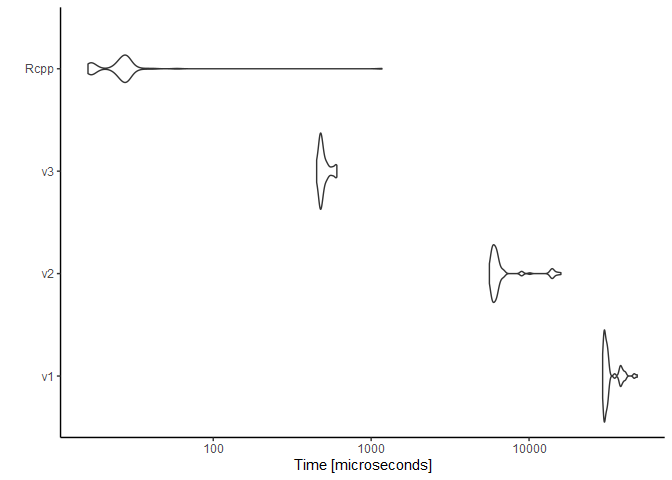
For n = 30000000, the C++ function completed in just under one second—about ten times faster than my fastest pure-R code. Worth it? Possibly not for this one-off exercise, but it’s interesting to note.

Day 16 - Ticket translation

The first thing we need to do is parse the input data. Everything can be grouped into three sections that are separated by blank lines. As each section is structured rather differently, it’s easier to treat them separately.

This is very much a job for the package tidyr. In my case I will process your ticket and nearby tickets together and the former will be denoted by a ticket_id of 0.

input <- readLines('input16.txt')

library(tidyr)
rules <- input[cumsum(!nchar(input)) < 1] %>%
  tibble(rules = .) %>%
  extract(rules,
          c('field_name', 'min1', 'max1', 'min2', 'max2'),
          '(.+): (\\d+)-(\\d+) or (\\d+)-(\\d+)',
          convert = TRUE)

tickets <- input[cumsum(!nchar(input)) > 0] %>%
  tibble(value = .) %>%
  subset(grepl('^\\d', value)) %>%
  transform(value = strsplit(value, ','),
            ticket_id = seq_along(value) - 1L) %>%
  unnest_longer(value, indices_to = 'field_id') %>%
  transform(value = as.integer(value))

Invalid tickets

Firstly we identify and add up the invalid values.

library(data.table)
setDT(tickets, key = 'ticket_id')
tickets[, valid_field := any(value %between% .(rules$min1, rules$max1) |
                               value %between% .(rules$min2, rules$max2)),
        by = .(ticket_id, field_id)]
tickets[(!valid_field), sum(value)]

[1] 19087

Bipartite matching

Filter out any tickets with invalid fields:

tickets[, valid_ticket := all(valid_field), by = ticket_id]
tickets <- tickets[(valid_ticket)]
tickets$valid_field <- tickets$valid_ticket <- NULL

Then try to work out which fields are which. For this I finally get to use a non-equi join in data.table. Also known as witchcraft.

rules_long <- rules %>%
  pivot_longer(min1:max2,
               names_to = c('.value', 'rule'),
               names_pattern = '([a-z]{3})([1-2])')
setDT(rules_long, key = 'field_name')

matched_fields <- rules_long[tickets[ticket_id > 0],
                             .(field_name, field_id),
                             allow.cartesian = TRUE,
                             on = .(min <= value, max >= value)]
ntickets <- length(unique(tickets$ticket_id)) - 1 # for own ticket
matched_fields[, all := .N >= ntickets, by = .(field_name, field_id)]

We have field names assigned to IDs, but it’s not immediately clear what is the unique solution that maps exactly one field name to one ID. In graph theory, this is a maximum bipartite matching and can be solved as a linear programme.

The igraph package has a dedicated function for this. It’s extremely fragile: if you forget to set the vertex types then it’ll crash your R session immediately and without explanation. The types need to indicate whether a vertex corresponds to a field name or an ID.

library(igraph)
g <- graph_from_data_frame(matched_fields[(all)])
V(g)$type <- rep(1:0, each = vcount(g) / 2)
matching <- max_bipartite_match(g)$matching
tickets[, field_name := matching[as.character(field_id)]]
tickets[grepl('^departure', field_name) & !ticket_id] -> departures
format(prod(departures$value), scientific = FALSE)

[1] "1382443095281"

Day 17 - Conway cubes

The idea will be to grow the size of our cube by 1 in each of the three dimensions, keeping all the data so far in the middle. Actually doing this seems terrible inefficient, so I will instead anticipate the final size (i.e. dims + 6 × 2) and pre-allocate this memory.

The rules are:

• if a cube is active and exactly 2 or 3 of its neighbours are also active, the cube remains active. Otherwise, it becomes inactive.
• if a cube is inactive but exactly three of its neighbours are active, the cube becomes active. Otherwise, the cube remains inactive.

This is basically like the convolution we applied in day 11, but with an extra dimension. In R, an array is a matrix with an arbitrary number of dimensions. We can also take advantage of the outer product %o% to pad the space with zeros initially.

Three dimensions

cubes <- do.call(rbind, strsplit(readLines('input17.txt'), '')) == '#'

conway3D <- function(cubes, n) {
  padded <- matrix(0, nrow(cubes) + 2 * n,
                      ncol(cubes) + 2 * n)
  padded[(n + 1):(n + nrow(cubes)),
         (n + 1):(n + ncol(cubes))] <- cubes
  pad1D <- c(rep(0, n + 1), 1, rep(0, n + 1))
  padded <- padded %o% pad1D
  I <- dim(padded)[1]
  J <- dim(padded)[2]
  K <- dim(padded)[3]
  state <- padded
  for (step in seq_len(n)) {
    new_state <- state
    for (i in 1:I)
      for (j in 1:J)
        for (k in 1:K) {
          is <- max(i - 1, 0):min(i + 1, I)
          js <- max(j - 1, 0):min(j + 1, J)
          ks <- max(k - 1, 0):min(k + 1, K)
          neighbours <- sum(state[is, js, ks])
          if (state[i, j, k]) {
            new_state[i, j, k] <- neighbours %in% 3:4
          } else {
            new_state[i, j, k] <- neighbours == 3
          }
        }
    state <- new_state
  }
  sum(state)
}

conway3D(cubes, 6)

[1] 375

Four dimensions

Add another dimension. All this means is that adding another level to the loop. To allocate space initially, in conway3D we take the outer product of the two-dimensional matrix with a vector of zeros with a one in the middle (pad1D). In conway4D the basic idea is the same, but this time we use a matrix of zeros with a one in the middle (pad2D).

conway4D <- function(cubes, n) {
  padded <- matrix(0, nrow(cubes) + 2 * n,
                      ncol(cubes) + 2 * n)
  padded[(n + 1):(n + nrow(cubes)),
         (n + 1):(n + ncol(cubes))] <- cubes
  pad2D <- matrix(0, 2 * n + 1, 2 * n + 1)
  pad2D[n + 1, n + 1] <- 1
  padded <- padded %o% pad2D
  I <- dim(padded)[1]
  J <- dim(padded)[2]
  K <- dim(padded)[3]
  L <- dim(padded)[4]
  state <- padded
  for (step in seq_len(n)) {
    new_state <- state
    for (i in 1:I)
      for (j in 1:J)
        for (k in 1:K)
          for (l in 1:L) {
            is <- max(i - 1, 0):min(i + 1, I)
            js <- max(j - 1, 0):min(j + 1, J)
            ks <- max(k - 1, 0):min(k + 1, K)
            ls <- max(l - 1, 0):min(l + 1, L)
            neighbours <- sum(state[is, js, ks, ls])
            if (state[i, j, k, l]) {
              new_state[i, j, k, l] <- neighbours %in% 3:4
            } else {
              new_state[i, j, k, l] <- neighbours == 3
            }
          }
    state <- new_state
  }
  sum(state)
}

conway4D(cubes, 6)

[1] 2192

A five-level nested loop is probably most R users’ idea of hell. However it runs in a couple of seconds, so presumably it’s what they actually expect you to do here. I wouldn’t expect this code to scale well without a rewrite in Rcpp (see day 15) or a sparse matrix/tensor library.

Day 18 - Operation order

In an R session, the standard order of arithmetic operations applies:

1 + 2 * 3 + 4 * 5 + 6

[1] 33

Ignoring Bidmas

But if we define our own arithmetic operators, then R will just read them from left to right with no ‘Bidmas’ (or ‘Bodmas’ or ‘Pemdas’) to override it.

local({
  `%+%` <- function(a, b) a + b
  `%*%` <- function(a, b) a * b
  1 %+% 2 %*% 3 %+% 4 %*% 5 %+% 6
})

[1] 71

It’s also possible to reassign the base + and * operators themselves (with great power comes great responsibility), but if you do this then it retains ordering, so that’s not so helpful for part 1.

For now we just need a way to swap out the expressions in the maths homework for our custom ones, then parse and evaluate the formulae.

maths <- function(expr) {
  `%+%` <- function(a, b) a + b
  `%*%` <- function(a, b) a * b
  expr <- gsub('\\+', '%+%', expr)
  expr <- gsub('\\*', '%*%', expr)
  eval(parse(text = expr))
}

maths('1 + 2 * 3 + 4 * 5 + 6')

[1] 71

homework <- readLines('input18.txt')
results <- sapply(homework, maths)
format(sum(results), scientific = FALSE)

[1] "50956598240016"

A new order

In part 2 it turns out that the order of arithmetic operations does matter, just that the precedence of addition is above multiplication. Now we can hijack R’s understanding of operation order for our own purposes. We’ll call it Bidams to represent our new order.

Bidams <- function(expr) {
  # Do not try this at home!
  `+` <- function(a, b) base::`*`(a, b)
  `*` <- function(a, b) base::`+`(a, b)
  expr <- gsub('\\+', 'tmp', expr)
  expr <- gsub('\\*', '+', expr)
  expr <- gsub('tmp', '*', expr)
  eval(parse(text = expr))
}

Bidams('1 + 2 * 3 + 4 * 5 + 6')

[1] 231

results2 <- sapply(homework, Bidams)
format(sum(results2), scientific = FALSE)

[1] "535809575344339"

Would you ever want to reassign low-level operators like this? Well, ggplot2 does it—by overloading the + you can join ggproto objects together. (However Hadley Wickham said they would have used a pipe, %>%, had they discovered that first).

Reassigning addition to another function is also a hilarious prank you can play on someone who never clears out their global workspace. It’ll teach them the value of starting with clean working environment.

Day 19 - Monster messages

Consider the first example rule set.

0: 1 2
1: "a"
2: 1 3 | 3 1
3: "b"

This could be written as a regular expression. Rules 1 and 3 are a and b respectively, so then rule 2 is 'ab|ba' and hence rule 0 is 'a(ab|ba)', which will match the strings 'aab' and 'aba' but not 'aaa' or 'bba'.

grepl('^a(ab|ba)$', c('aab', 'aba', 'aaa', 'bba'))

[1]  TRUE  TRUE FALSE FALSE

The tricky bit is how to build the regex from a set of rules programmatically. Let’s look at the more complicated example.

0: 4 1 5
1: 2 3 | 3 2
2: 4 4 | 5 5
3: 4 5 | 5 4
4: "a"
5: "b"

In the first step, we notice that rules 4 and 5 are single characters, so we can simply replace all 4s and 5s with the letters a and b (dropping the quotation marks for now). We obtain:

0: a 1 b
1: 2 3 | 3 2
2: a a | b b
3: a b | b a
4: "a"
5: "b"

Then we see that rules 2 and 3 no longer contain any numerical IDs, so we can slot them into place in rule 1:

0: a 1 b
1: (a a | b b) (a b | b a) | (a b | b a) (a a | b b)
2: a a | b b
3: a b | b a
4: "a"
5: "b"

Hence insert the rule 1 into rule 0 and we are done.

Regex generator

Import the data:

library(magrittr)
input <- readLines('input19.txt')
rules <- input[cumsum(!nchar(input)) < 1] %>%
  strsplit(': ') %>% do.call(rbind, .) %>%
  as.data.frame %>% setNames(c('id', 'rule'))
messages <- input[cumsum(!nchar(input)) > 0][-1]

Then implement the algorithm, which works like this:

1. For every rule, replace any integers in the pattern with the rules corresponding to those integer IDs.
2. Repeat until none of the patterns contain any integers.

For it to be a valid regular expression, we should also ignore the spaces between the terms, but we don’t need to do this until the very end.

library(stringr)
make_regex_bounded <- function(rules, max_length = Inf) {
  rules %<>%
    transform(regex = str_remove_all(rule, '["]')) %>%
    transform(char_only = str_detect(regex, '\\d', negate = TRUE))
  
  while( any(!rules$char_only) ) {
    rules %<>%
      transform(regex = str_replace_all(regex,
      pattern =  '\\d+',
      replacement = function(d) {
        rule_d <- rules$regex[rules$id == d]
        len <- str_count(rule_d, '\\([^)]*\\)')
        if (len > max_length)  # for part 2
          return('x')
        if (!str_detect(rule_d, '\\|'))
          return(rule_d)
        sprintf('(?:%s)', rule_d)
      }
    )) %>%
      transform(char_only = str_detect(regex, '\\d', negate = TRUE))
  }
  
  str_remove_all(rules$regex[1], ' ')
}

All that remains is a bit of housekeeping: for an exact match, the regular expression should start and end with ^ and $ anchors, otherwise it risks matching substrings of longer messages.

matching_messages <- function(rules, messages) {
  longest <- max(nchar(messages))
  regex <- sprintf('^%s$', make_regex_bounded(rules, longest))
  matches <- str_detect(messages, regex)
  sum(matches)
}

matching_messages(rules, messages)

[1] 285

Loops and bounds

The number of possible rules might be infinite, but rules are monotonically increasing in length, whereas our input messages are of finite length. Thus the only change we need to make is to impose a cap on the maximum message length, deleting any parts of rules that are longer than this, as they will never match any of our messages.

We incorporated this with a maximum message length in our function make_regex_bounded. It isn’t necessary for part 1 but it will cut off any runaway rules in part 2. It does this by replacing overlong patterns with the literal letter x, which (we assume) doesn’t appear in any of our messages so will never match.

rules2 <- within(rules, {
  rule[id == '8'] <- '42 | 42 8'
  rule[id == '11'] <- '42 31 | 42 11 31'
})

matching_messages(rules2, messages)

[1] 412

I am not sure what the best way is to count the possible lengths of matches to a regular expression but in this case I used '\([^)]*\)', which detects pairs of brackets that do not contain other brackets. The shortest possible pattern length is one (or maybe two because I didn’t enclose single letters in brackets) so this provides a reasonable lower bound.

Day 20 - Jurassic jigsaw

To match up the puzzle edges, we need to find an edge of each puzzle piece that matches up with at least one other puzzle piece. It’s possible that there might be multiple candidates, but presumably there is only one way to fit the entire jigsaw together.

library(dplyr)
tiles <- tibble(input = readLines('input20.txt')) %>%
    mutate(is_tile_id = grepl('Tile', input),
           tile_id = input[which(is_tile_id)[cumsum(is_tile_id)]],
           tile_id = as.integer(gsub('\\D', '', tile_id))) %>%
    subset(!is_tile_id & nchar(input) > 0, select = -is_tile_id) %>%
    group_by(tile_id) %>%
    summarise(tile_matrix = list(input),
              tile_matrix = lapply(tile_matrix, strsplit, ''),
              tile_matrix = lapply(tile_matrix, do.call, what = rbind))

We don’t care about the interior data of each tile. And since the entire puzzle can be rotated, the solution will be non-unique unless we fix the first tile in place and then fit the other tiles around it.

Possible transformations are

• Flip horizontally, or matrix[, ncol(matrix):1]
• Flip vertically, or matrix[nrow(matrix):1, ]
• Rotate 90°, or t(matrix)

Finding corner pieces

If it’s a corner piece, the tile will be joined to exactly two other tiles. If it’s an edge piece, it will join three other tiles and if it’s an interior piece then it will join four others.

library(tidyr)
dims <- dim(tiles$tile_matrix[[1]])
edges <- tiles %>%
  mutate(top = lapply(tile_matrix, '[', 1, 1:dims[2]),
         bottom = lapply(tile_matrix, '[', dims[1], 1:dims[2]), 
         left = lapply(tile_matrix, '[', 1:dims[1], 1),
         right = lapply(tile_matrix, '[', 1:dims[1], dims[2])) %>%
  select(-tile_matrix) %>%
  mutate_at(vars(top:right), sapply, paste, collapse = '') %>%
  pivot_longer(top:right) %>%
  bind_rows(mutate(., name = paste0(name, 'rev'),
                   value = stringi::stri_reverse(value)))

No point in reversing both the piece and that to which it is matched. So we fix the first piece in place and rotate the other pieces to fit. A corner piece is any piece that attaches to two other pieces, where those two other pieces attach to three other pieces. The actual joining can be done with a SQL-like dplyr::inner_join:

library(magrittr)
jigsaw <- edges %>%
  inner_join(filter(., tile_id != first(tile_id),
             !grepl('rev', name)), ., by = 'value') %>%
  filter(tile_id.x != tile_id.y) %>%
  add_count(tile_id.x, name = 'n.x') %>%
  add_count(tile_id.y, name = 'n.y') 
  
corner <- jigsaw %$%
  union(tile_id.x[n.x == 2 & n.y == 3],
        tile_id.y[n.y == 2 & n.x == 3])

prod(corner) %>% format(scientific = FALSE)

[1] "15670959891893"

As you can see I don’t care how the image as a whole fits together—the code just work out which tiles are valid corner pieces.

A more complex approach.

And now for something completely different. Storing these as matrices seems awfully inefficient, and coming up with eight different orientations of the tiles is a bit of a slog. What if we could store, say, the # symbols as their indices alone, in a sparse, complex number representation?

Thus we make the solution a bit like day 12 by treating rotations and translations as complex arithmetic.

transformations <- expand.grid(flip = c(FALSE, TRUE),
                               rotate = 1i^(1:4),
                               tile_id = unique(tiles$tile_id))

complex_tiles <- tiles %>%
  # Convert to complex coordinates of the '#' symbols.
  mutate(hashes = lapply(tile_matrix, function(x) which(x == '#', arr.ind = T)),
         hashes = lapply(hashes, function(x) x[, 1] + x[, 2] * 1i)) %>%
  select(-tile_matrix) %>%
  # Transform by flipping (complex conjugate) and rotating (* i).
  left_join(transformations, by = 'tile_id') %>%
  unnest_longer(hashes) %>%
  mutate(hashes2 = ifelse(flip, Conj(hashes) * rotate, hashes * rotate),
         hashes2 = (Re(hashes2) %% (dims[2] + 1)) +
           (Im(hashes2) %% (dims[1] + 1)) * 1i,
         # Cannot do joins on complex numbers:
         rotate = Arg(rotate) %% (2 * pi)) %>%
  group_by(tile_id, flip, rotate) %>%
  summarise(hashes = list(sort(hashes2)), .groups = 'drop')

complex_edges <- complex_tiles %>%
  mutate(top =    lapply(hashes, function(h) Im(h)[Re(h) == 1]),
         left =   lapply(hashes, function(h) Re(h)[Im(h) == 1]),
         right =  lapply(hashes, function(h) Re(h)[Im(h) == dims[1]]),
         bottom = lapply(hashes, function(h) Im(h)[Re(h) == dims[2]])) %>%
  select(-hashes) %>%
  mutate_at(vars(top:bottom), sapply, paste, collapse = ' ')

# Find where the edges match between tiles.
complex_edges %<>%
  inner_join(., ., by = c(right = 'left'),
            suffix = c('', '.right')) %>%
  filter(tile_id != tile_id.right)

And here is the solution to part 1, again.

complex_edges %>%
  count(tile_id) %>% filter(n == min(n)) %$%
  prod(tile_id) %>% format(scientific = FALSE)

[1] "15670959891893"

Arranging the tiles

Now we are actually supposed to build up the image and look for patterns in it (discarding the edges) that look like this sea monster:

                  # 
#    ##    ##    ###
 #  #  #  #  #  #   

Our approach starts at the top-left of the image and works to the right. When we get to the end of a row of tiles, we rotate the first tile of the previous row so that ‘below’ becomes ‘right’ and we can get the first tile of the next now (rotating back again to the correct orientation). Then we convert the complex indices into a matrix of hashes.

complex_tiles %<>%
  mutate(hash_content = lapply(hashes, function(h) h[Re(h) > 1 & Im(h) > 1 &
                                                       Re(h) < dims[2] &
                                                       Im(h) < dims[1]]))

image_row <- function(start) {
  img <- NULL
  current_tile <- start
  repeat {
    img <- img %>%
      bind_rows(left_join(current_tile, complex_tiles))
    if ( is.na(current_tile$tile_id.right) )
      break
    next_tile <- current_tile %>%
      select(tile_id = tile_id.right,
             rotate = rotate.right,
             flip = flip.right) %>%
      left_join(complex_edges, by = c('tile_id', 'rotate', 'flip'))
    
    current_tile <- next_tile
  }
  img
}

# Make sure nothing can appear above/left of start.
row_start <- complex_edges %>%
  add_count(top, name = 'n_top') %>%
  add_count(left, name = 'n_left') %>%
  filter(n_top == 1, n_left == 1) %>%
  slice(2) %>% select(-n_top, -n_left)

grid_size <- sqrt(nrow(tiles))
img_data <- tibble()
for (row in 1:grid_size) {
  img_data %<>% bind_rows(image_row(row_start))
  # Rotate to get the next row start:
  row_start %<>%
    mutate(rotate = (rotate + pi / 2) %% (2 * pi),
           flip = flip) %>%
    select(tile_id, flip, rotate) %>%
    left_join(complex_edges) %>%
    transmute(tile_id = tile_id.right,
              flip = flip.right,
              rotate = (rotate.right - pi / 2) %% (2 * pi)) %>%  # undo rotation
    left_join(complex_edges)
}

stopifnot('Image is missing tiles' = nrow(img_data) == nrow(tiles))

image <- img_data %>%
  select(tile_id, hashes) %>%
  mutate(row = rep(1:grid_size, each = grid_size),
         col = rep(1:grid_size, times = grid_size)) %>%
  unnest_longer(hashes) %>%
  mutate(hashes = hashes + (dims[1] - 1) * ((col - 1) * 1i + (row - 1)),
         i = Im(hashes), j = Re(hashes))

image <- img_data %>%
  select(tile_id, hashes = hash_content) %>%
  mutate(row = rep(1:grid_size, each = grid_size),
         col = rep(1:grid_size, times = grid_size)) %>%
  unnest_longer(hashes) %>%
  mutate(hashes = hashes + (dims[1] - 2) * ((col - 1) * 1i + (row - 1)),
         i = Im(hashes), j = Re(hashes))

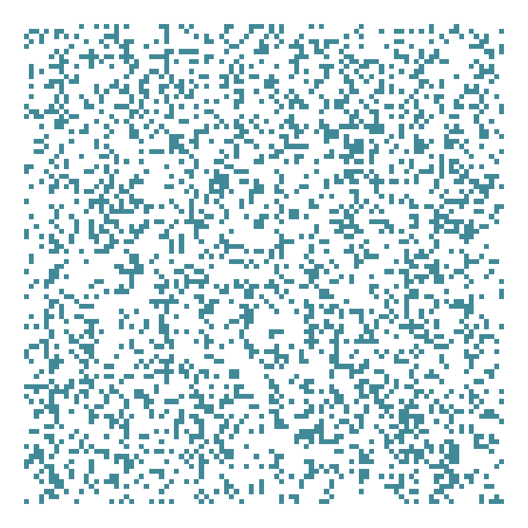
Here’s what the scene looks like:

Now let’s go monster hunting.

monster <- c('                  # ',
             '#    ##    ##    ###',
             ' #  #  #  #  #  #   ')
monster <- do.call(rbind, strsplit(monster, '')) == '#'
monster_ids <- as.data.frame(which(monster, arr.ind = TRUE))

monster_search <- function(image, monster) {
  monsters <- NULL
  monster_ids <- as.data.frame(which(monster, arr.ind = TRUE))
  for (i in 0:(max(image$i) - max(monster_ids$row)))
    for (j in 0:(max(image$j) - max(monster_ids$col))) {
      shifted_monster <- transform(monster_ids, i = row + i, j = col + j)
      join <- semi_join(shifted_monster, image, by = c('i', 'j'))
      if (nrow(join) == nrow(monster_ids))
        monsters <- bind_rows(monsters, shifted_monster[, c('i', 'j')])
    }
  monsters
}

for (rotation in 1i^(1:4)) {
  for (flip in 0:1) {
    transformed <- image %>%
        mutate(hashes = rotation * if (flip) Conj(hashes) else hashes,
               i = Im(hashes) %% (grid_size * dims[1] - 2),
               j = Re(hashes) %% (grid_size * dims[2] - 2))
    results <- monster_search(transformed, monster)
    if (length(results))
      break
  }
  if (length(results))
    break
}

cat(sprintf('Found %d monsters; water roughness is %d',
            nrow(results) / nrow(monster_ids),
            nrow(image) - nrow(results)))

Found 38 monsters; water roughness is 1964

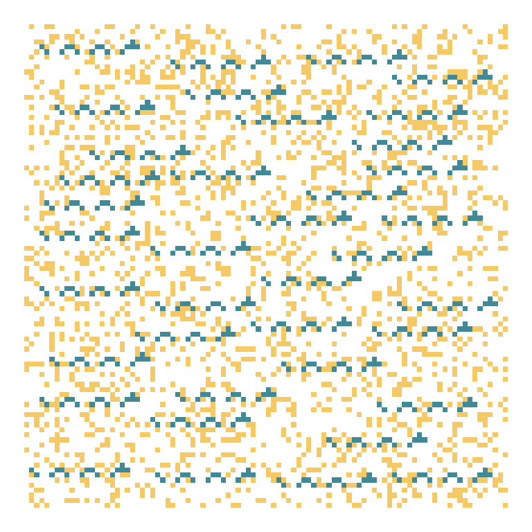
Where are they on the map?

ggplot(transformed) +
  aes(j, i) +
  geom_tile(fill = '#f5c966') +
  geom_tile(data = results, fill = '#418997') +
  scale_y_reverse() +
  theme_void()

This puzzle was a real slog!

I got waylaid for a while by the fact you can’t do table joins on complex number columns in dplyr. My workaround was to convert the rotations to their angles in radians (using Arg()), but in retrospect it would have been more robust to convert the numbers to string, or just to give each tile rotation a unique ID.

Day 21 - Allergen assessment

Each allergen is found in exactly one ingredient.

input <- readLines('input21.txt')

library(tidyr)
ingredients <- tibble(input = input) %>%
  tidyr::extract(input, c('ingredient', 'allergen'),
                 '(.+) \\(contains (.+)\\)') %>%
  transform(ingredient = strsplit(ingredient, ' '),
            allergen = strsplit(allergen, ', '))

Allergen intersection

We can find the risky ingredients via an intersection operation between recipes that contain each allergen.

library(dplyr)
risky_foods <- ingredients %>%
  unnest_longer(allergen) %>%
  group_by(allergen) %>%
  summarise(ingredient = Reduce(intersect, ingredient))

Part 1 asks us to count up the number of times that non-risky foods appear.

ingredients %>%
  unnest_longer(ingredient) %>%
  count(ingredient) %>%
  anti_join(risky_foods) %>%
  pull(n) %>% sum

[1] 2786

Bipartite food pairing

This is a bipartite graph theory problem, just as in day 16.

library(igraph)
g <- graph_from_data_frame(risky_foods)
V(g)$type <- V(g)$name %in% risky_foods$ingredient
matching <- max_bipartite_match(g)$matching

matching[V(g)$type] %>%
  sort %>% names %>%
  paste(collapse = ',')

[1] "prxmdlz,ncjv,knprxg,lxjtns,vzzz,clg,cxfz,qdfpq"

Refreshingly straightforward.

Day 22 - Crab combat

Combat

Games are independent of one another until cards from previous games come back into play. Therefore, if player 1 has $n$ cards and player2 has $m$ cards, we can simulate the first $\min(n, m)$ rounds in parallel.

combat <- function(p1, p2) {
  if (!length(p1)) return(p2)
  if (!length(p2)) return(p1)
  length(p1) <- length(p2) <- max(length(p1), length(p2))
  win1 <- p1 > p2
  result1 <- c(rbind(p1[win1], p2[win1]))
  result2 <- c(rbind(p2[!win1], p1[!win1]))
  output1 <- c(p1[is.na(win1)], result1)
  output2 <- c(p2[is.na(win1)], result2)
  combat(output1[!is.na(output1)], output2[!is.na(output2)])
}

Test on the example data:

ex1 <- c(9, 2, 6, 3, 1)
ex2 <- c(5, 8, 4, 7, 10)
example <- combat(ex1, ex2)
sum(rev(example) * seq_along(example))

[1] 306

Now read in the puzzle input and simulate for part 1.

input <- as.integer(readLines('input22.txt'))
deck <- matrix(input[!is.na(input)], ncol = 2)
result <- combat(deck[, 1], deck[, 2])
sum(rev(result) * seq_along(result))

[1] 30138

Apparently, I wasn’t supposed to do the first part with a recursion and should have used a while loop, instead. I have to fix this in the second part, as we shall see.

Recursive combat

For the next round we actually need a recursion.

The rules are as follows:

1. If this exact round has happened before (during this game), we stop and player 1 automatically wins the game, to prevent an infinite recursion.
2. If each player’s deck has more cards than the value of their latest draw, copy the next value cards and play a (recursive) sub-game to determine the winner of this round.
3. Otherwise, the player with the higher-value card wins the round.

To keep track of already-played rounds, I’m going to store the deck configuration as a string. However, you could also take a hint from submitting the answer to part 1: the sum of the deck multiplied by its indices is unique.

For part 2 it’s not as easy to take advantage of vectorisation, because even though a win or a loss is still a binary value, it depends on the result of the previous game (in the event that it goes to a sub-game).

Since the outer function needs to return scores (for submitting as our puzzle answer) but the inner functions need only to say who won each match, we can return the final deck as a positive vector if it was player 1 who won, and negated if it was player 2.

Initially I tried to wrap up my previously-recursive function for part 1 in another recursion.

recursive_recursive_combat <- function(p1, p2, subgame = FALSE,
                                       played = NULL) {
  if (!length(p1)) return(-p2)
  if (!length(p2)) return(p1)
  # If player 1 holds highest card, skip the sub-game.
  if (subgame & (max(p1) > max(p2))) return(p1)
  
  # Has this game already been played? If so, player 1 wins.
  config <- paste(p1, p2, collapse = ',', sep = '|')
  if (config %in% played) return(p1)
  played <- c(played, config)
  
  # Does each player have as many cards as their last dealt card value?
  # If so, play a sub-game with a copy of the next {value} cards.
  if (p1[1] < length(p1) & p2[1] < length(p2)) {
    win1 <- all( recursive_recursive_combat(head(p1[-1], p1[1]),
                                            head(p2[-1], p2[1]),
                                            subgame = TRUE) > 0)
  } else win1 <- p1[1] > p2[1]
  
  result1 <- c(p1[-1], p1[1][win1], p2[1][win1])
  result2 <- c(p2[-1], p2[1][!win1], p1[1][!win1])
  
  recursive_recursive_combat(result1, result2, subgame, played)
}

This works OK on the small example dataset. Testing on the example data, a negative score indicates it is the crab who wins:

example2 <- recursive_recursive_combat(ex1, ex2, F)
sum(rev(example2) * seq_along(example2))

[1] -291

But on the test inputs, it became clear that a recursion within a recursion was not such a great idea. The deeply nested recursion causes a stack overflow. (Edit: at least, it did before I added the sub-game skipping trick, described below.)

result2 <- recursive_recursive_combat(deck[, 1], deck[, 2])
sum(rev(result2) * seq_along(result2))

[1] 31587

Rewriting the main game as a loop is probably better coding practice. This is the equivalent non-doubly-recursive version:

recursive_combat <- function(p1, p2, subgame = FALSE) {
  if (subgame & (max(p1) > max(p2))) return(p1)
  played <- NULL
  while (length(p1) & length(p2)) {
    config <- paste(p1, p2, collapse = ',', sep = '|')
    if (config %in% played) return(p1)
    played <- c(played, config)
    
    if (p1[1] < length(p1) & p2[1] < length(p2)) {
      win1 <- all( recursive_combat(head(p1[-1], p1[1]),
                                    head(p2[-1], p2[1]),
                                    subgame = TRUE) > 0 )
    } else win1 <- p1[1] > p2[1]
    
    result1 <- c(p1[-1], p1[1][win1], p2[1][win1])
    result2 <- c(p2[-1], p2[1][!win1], p1[1][!win1])
    
    p1 <- result1
    p2 <- result2
  }
  
  if (!length(p1)) return(-p2)
  p1
}

result2 <- recursive_combat(deck[, 1], deck[, 2])
sum(rev(result2) * seq_along(result2))

[1] 31587

Writing recursive functions just to avoid loops is a bad idea because it can result in nesting so deep that a stack overflow occurs, and it’s just as easy to write a while loop for the outer part of this algorithm.

However, since I originally solved this problem, I came across a trick that not only prevents a stack overflow, but it speeds up the algorithm significantly by avoiding a large amount of unnecessary computation (both for the double recursion and outer-loop versions).

Specifically: in any sub-game, if player 1 holds the highest card, they are guaranteed to win. This is because they will never hand this maximum card over to player 2, so the sub-game will just continue until either player 2 loses, or a loop occurs, in which case player 1 wins by default according to rule 1.

(The maximum card will never trigger a sub-sub-game, because the maximum value in a set of distinct natural numbers is always greater than or equal to the size of that set. You could even use this fact to skip the main game of recursive combat—if you didn’t need to know the final score.)

By checking before each sub-game if player 1 holds the maximum card, and skipping the sub-game if it is a foregone conclusion, a huge amount of computation can be avoided, and it may even reduce the call stack such that recursive_recursive_combat() works without error (at least on my input data).

According to microbenchmark, this trick cuts my run time from around 34 seconds to just 250 milliseconds on the full data (and the loop is a few ms faster than the double recursion).

Also: the crab lost.

Day 23 - Crab cups

Ten moves

In the first part, the key bit to figure out is how to cycle through a vector, such that if you reach either the maximum index or maximum value, the following index/value loops back round to the start.

You can do this with modular arithmetic, for which I wrote a utility function idx(), which makes the rest of the code easier to read. R indices and the values on the cups both start at 1 (rather than 0) so you need to subtract 1, get the modulo and then add 1 again.

crab_cups <- function(circle, moves = 10) {
  ncups <- length(circle)
  idx <- function(i) 1 + (i - 1) %% ncups
  i <- 1
  for (iter in 1:moves) {
    current <- circle[idx(i)]
    grab <- circle[idx(seq(i + 1, i + 3))]
    dest <- idx(current - 1:4)
    dest <- dest[which.min(dest %in% grab)]
    next_circle <- setdiff(circle, grab)
    next_circle <- append(next_circle, grab,
                          after = which(next_circle == dest))
    circle <- next_circle
    i <- which(circle == current) + 1
  }
  circle
}

labels <- function(circle) {
  n <- length(circle)
  i1 <- which(circle == 1)
  result <- circle[1 + (i1 + 0:(n - 2)) %% n]
  paste(result, collapse = '')
}

example <- crab_cups(c(3, 8, 9, 1, 2, 5, 4, 6, 7))
labels(example)

[1] "92658374"

Another helper function, labels(), deals with rotating the vector so we get all the values after the cup labelled with a 1.

input <- c(9, 7, 4, 6, 1, 8, 3, 5, 2)
result <- crab_cups(input, 100)
labels(result)

[1] "75893264"

Ten million moves

In principle we’ve just been asked to add a load of cups and run the same thing again, but clearly this won’t scale well over ten million moves with a million cups. There must be a trick here to reduce the computational load, but what is it? Ten million moves is a tiny amount relative to the number of possible orderings (which is $1000000!$) so it seems unlikely we’ll hit a loop.

There is no way to skip steps as in yesterday’s problem. Instead, we look at how the circle itself is stored.

To avoid shrinking and resizing the vector of values, or updating many elements’ values or positions in place, we can take advantage of a data structure known as a linked list. In a linked list, positions of elements are described by relative rather than absolute indices.

We can store the cups as a linked list where each label is linked to the label of the cup immediately preceding (anti-clockwise to) it in the circle. Then, at each iteration, the only nodes that need updating are the current cup, the destination cup and those cups that are immediately adjacent to the three we pick up.

There is no specific class for linked lists in base R; instead you can use an ordinary vector where the index of each element corresponds to the label of the previous one. An nifty one-liner for this is c(x[-1], x[1])[order(x)], which you can see implemented below.

linked_cups <- function(circle, moves = 10, terms = 9) {
  ncups <- length(circle)
  stopifnot(terms <= ncups)
  # Linked list where each index is the label of the preceding cup.
  lnklst <- c(circle[-1], circle[1])[order(circle)]
  current <- circle[1]
  for (iter in 1:moves) {
    # Pick the 3 next cups.
    grab1 <- lnklst[current]
    grab2 <- lnklst[grab1]
    grab3 <- lnklst[grab2]
    # Choose destination.
    dest <- 1 + (current - 1:4 - 1) %% ncups
    dest <- dest[which.min(dest %in% c(grab1, grab2, grab3))]
    # Lift out the 3 cups.
    lnklst[current] <- lnklst[grab3]
    # Slot in the 3 cups.
    lnklst[grab3] <- lnklst[dest]
    lnklst[dest] <- grab1
    # Move clockwise by 1.
    current <- lnklst[current]
  }
  
  # Convert back into a vector of labels for output.
  cups <- integer(terms)
  cups[1] <- 1
  for (i in 2:terms) cups[i] <- lnklst[cups[i-1]]
  cups
}

result2 <- linked_cups(c(input, 10:1e6), 1e7, terms = 3)
prod(result2)

[1] 38162588308

As a linked list has no absolute start or end point, the function above just returns the few terms immediately after 1 in the circle, which is all we need for the puzzle solution.

A more R-like solution might be just to use a named vector/list. Something like:

linked_list <- setNames(c(circle[-1], circle[1]), circle)

though you have to be careful with this because linked_list['1'] is not the same thing as linked_list[1]. The former means ‘the label after label 1’ whereas the latter just gives the first element of the vector (which could be something else entirely, unless the vector were sorted by its names). An advantage of a named vector is that you can have any labels you like, including zeros, negative numbers, non-integers or strings.

However, for this particular example, the conversion back and forth from integer to character makes a named vector/list slower than the index-based solution above.

Day 24 - Lobby layout

The first challenge in this puzzle is parsing the input, which has no delimiters between directions. As the directions are e, se, sw, w, nw and ne, there aren’t any directions that are a partial match for any other direction. So we can use a regular expression to split up the input.

That is, every direction ends with either 'e' or 'w', and starts with any other cardinal direction. So we break up the input strings as follows using a regular expression lookbehind and lookahead, effectively making a custom word boundary:

input <- readLines('input24a.txt')
input <- stringi::stri_split(input, regex = '(?<=[ew])(?=.)')

Hexagonal coordinates

The next thing we need is a coordinate system. An ordinary 2-dimensional lattice in Cartesian coordinates doesn’t quite do the trick, because we can move in six directions, not just four.

We need an hexagonal coordinate system and one way of representing this is in three-dimensional space $(x, y, z)$ where $x + y + z = 0$ for every point at the origin. Then axial offsets are:

• origin - (0, 0)
• ne - (1, -1)
• e - (1, 0)
• se - (0, 1)
• sw - (-1, 1)
• w - (-1, 0)
• nw - (0, -1)

It’s not so easy to visualise this, but it should be easy enough to implement in R. Let zero represent a white tile and one represent black, and construct a coordinate system $(x, y, z)$ defined as above.

library(dplyr)
hex_coords <- tibble(
  dir = c('ne', 'e', 'se', 'sw', 'w', 'nw'),
  x = c(1, 1, 0, -1, -1, 0),
  y = c(-1, 0, 1, 1, 0, -1)
)

floor_pattern <- tibble(
  row = rep(seq_along(input), lengths(input)),
  dir = unlist(input)
) %>%
  left_join(hex_coords, by = 'dir')

Now we have a data frame containing our instructions, we need to follow them, which amounts to taking the cumulative sum of the individual directions.

I got very confused by this by not reading the puzzle properly. In particular:

Each line in the list identifies a single tile that needs to be flipped by giving a series of steps starting from a reference tile in the very center of the room.

Initially I assumed that every tile you walk on as you go along the line also got flipped. But it’s only the very end of each line that needs flipping.

Thus the solution is a simple split-apply-combine operation. We add up the coordinates to find out which tile each line of the input refers to. Then we count how many times each tile appears, and our result is the number of tiles that appear an odd number of times.

black_tiles <- floor_pattern %>%
  group_by(row) %>%
  summarise(x = sum(x), y = sum(y)) %>%
  count(x, y) %>%
  filter(n %% 2 == 1)

nrow(black_tiles)

[1] 10

Conway tiles

The second part of this puzzle is essentially similar to day 17. We can adapt that code for this puzzle, or take a slightly different approach.

A reminder, the rules are:

• any black tile with zero or more than 2 black tiles immediately adjacent to it is flipped to white.
• any white tile with exactly 2 black tiles immediately adjacent to it is flipped to black.

Here is a (slow) dataframe-based approach that uses lots of joins.

full_grid <- expand.grid(i = -100:100,
                         j = -100:100) %>%
  left_join(black_tiles, by = c(i = 'x', j = 'y')) %>%
  mutate(n = !is.na(n)) %>%
  rename(black = n) %>%
  tidyr::crossing(hex_coords) %>%
  mutate(neighbour_x = i + x,
         neighbour_y = j + y) %>%
  select(-x, -y)

for (day in 1:100) {
  full_grid <- full_grid %>%
    inner_join(full_grid %>% distinct(i, j, black),
               by = c(neighbour_x = 'i', neighbour_y = 'j'),
               suffix = c('', '.y')) %>%
    add_count(i, j, wt = black.y) %>%
    mutate(black = ifelse(black, n == 1 | n == 2, n == 2)) %>%
    select(-black.y, -n)
}

full_grid %>%
  filter(black) %>%
  distinct(i, j) %>%
  nrow

[1] 2208

It’s not very efficient, but it works!

Here is what the grid looks like after 100 days (except the actual pattern would be hexagonal).

Faster approach?

I’ve been inspired by Thomas Loock on Twitter, whose concise solution takes advantage of Python’s defaultdict data structure. This is like an ordinary Python dictionary, but if you try to extract a key that doesn’t exist, it returns a default value (e.g. false) rather than throwing an error.

Can we implement something similar in R?

The nearest R equivalent to a Python dictionary is a named list. But is there an R equivalent to a defaultdict? Well, a few things, actually. In fact, most R data structures will return either NA (vectors) or NULL (lists) if the key or index is missing. The exception to this is arrays/matrices, which throw a subscript out of bounds error if that dimension doesn’t exist.

Here is an R translation. The dictionary delta can be a named list. Looping over lines of an open file is probably not very R-like, so we use the regex from earlier to parse the input. Similarly, most of the rest of the initial while loop can be a one-liner, leaving just the issue of getting rid of tiles flipped back to white.

delta <- list(w = c(-1, 0), e = c(1, 0), ne = c(0, 1), nw = c(-1, 1),
              se = c(1, -1), sw = c(0, -1))
file <- readLines('input24.txt')
input <- stringi::stri_split(file, regex = '(?<=[ew])(?=.)')
tiles <- sapply(input, function(x) Reduce('+', delta[x]))
tiles <- setNames(as.data.table(t(tiles)), c('x', 'y'))
tiles <- tiles[j = .(n = .N), by = .(x, y)]

cat('Part 1:', tiles[n %% 2 == 1, .N])

Part 1: 473

deltaDT <- setNames(as.data.table(do.call(rbind, delta)), c('dx', 'dy'))
for (day in 1:100) {
  tiles <- tiles[n %% 2 == 1]
  neighbours <- setDT(tidyr::crossing(tiles, deltaDT))
  neighbours[, x := x + dx][, y := y + dy]
  neighbours <- neighbours[, .(nbrs = .N), by = .(x, y)]
  tiles <- merge(tiles, neighbours, all = TRUE)
  # If is.na(n), tile is white.
  # If is.na(nbrs), tile has no neighbours.
  tiles[!is.na(n), new := !is.na(nbrs) & nbrs > 0 & nbrs < 3]
  tiles[is.na(n),  new := !is.na(nbrs) & nbrs == 2]
  tiles[, n := new][, new := NULL][, nbrs := NULL]
}

cat('Part 2:', tiles[n %% 2 == 1, .N])

Part 2: 4070

Once into part 2, it’s back to a tabular solution, but this data.table implementation is much faster than the dplyr version originally implemented above.

Day 25 - Combo breaker

1. Set value to itself multiplied by the subject number (7).
2. Set the value to itself modulo 20201227.
3. Repeat loopsize times until we get the original value again.

Once we have the loop size for one device, change the subject to the public key of the other device and run the loop that many times to get the encryption key. Run it both ways (using the other loop size and the other public key) to verify the same encryption key comes out.

I wrote the same function to do both tasks. The default publickey and loop size are infinite. Pass it just a public key and it will give you the loop size. Pass it a subject (from a public key) and a loop size and it will return the encryption key.

decrypt <- function(publickey = -Inf, loop = Inf, subject = 7) {
  stopifnot(is.finite(publickey) + is.finite(loop) == 1)
  value <- subject
  iter <- 1
  repeat {
    if (value == publickey) return(iter) # Loop size
    if (iter >= loop) return(value)      # Encryption key
    value <- (value * subject) %% 20201227
    iter <- iter + 1
  }
}

On the example data:

decrypt(subject = 17807724, loop = decrypt(publickey = 5764801))

[1] 14897079

decrypt(subject = 5764801, loop = decrypt(publickey = 17807724))

[1] 14897079

And the puzzle inputs:

input <- as.double(readLines('input25.txt'))
key1 <- decrypt(subject = input[2], loop = decrypt(input[1]))
key2 <- decrypt(subject = input[1], loop = decrypt(input[2]))
stopifnot(key1 == key2)
key1

[1] 545789

Running both isn’t strictly necessary but it’s good to verify they give the same result.

An even shorter version, once again inspired by Thomas Loock, who recognised you only need a single loop:

decrypt2 <- function(card, door) {
  val <- c(subj = 7, key = door)
  while(val['subj'] != card)
    val <- (val * c(7, door)) %% 20201227
  val['key']
}

input <- as.double(readLines('input25.txt'))
do.call(decrypt2, as.list(input))

   key 
545789 

Or, if you really enjoy abusing R’s assignment operator (<-), you can do everything in two lines, plus one to print the result. It even features a gratuitous while loop that does nothing. For code golf enthusiasts only!

val <- c(subj = 7, key = (input <- as.double(readLines('input25.txt')))[2])
while((val <- (val * c(7, input[2])) %% 20201227)['subj'] != input[1]) NULL
val['key']

   key 
545789 

Merry Christmas!