Part 2 Mixed effects models
A mixed model, also known as a hierarchical or multilevel model, in general contains both random (subject or group level) and fixed (population level) effects.
2.1 Restricted maximum likelihood
The standard way for fitting mixed effects models in R is lme4 (Bates et al. 2020), which estimates the parameters via restricted maximum likelihood optimization.
A canonical example dataset is sleepstudy, bundled with the package, which records reaction times each day for 18 subjects restricted to three hours of sleep per night.
The data are visualised in Figure 2.1.
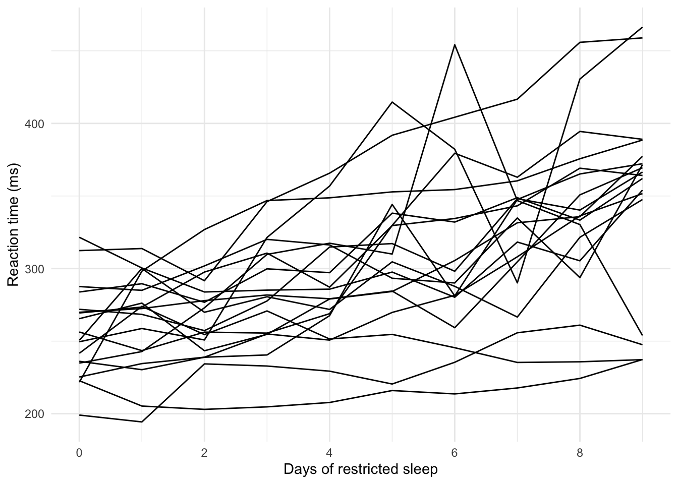
Figure 2.1: Average reaction time per day (ms) for 18 subjects in a sleep deprivation study. Each line represents one subject
Overall, we would probably expect reaction times to increase as the subjects become more sleep-deprived. But some subjects surely will have had faster reaction times than others, even before the study began. This is modelled using a random intercept coefficient. Meanwhile, we might assume each day of sleep deprivation results in the same increase in reaction time for every participant, in which case a common, fixed slope coefficient is appropriate. However, if instead we thought the daily effect of sleep deprivation varied between subjects, we could fit random slopes (as well as the random intercept).
In lme4 syntax, the random intercept model is
which yields the following summary output.
Linear mixed model fit by REML ['lmerMod']
Formula: Reaction ~ Days + (1 | Subject)
   Data: sleepstudy

REML criterion at convergence: 1786.5

Scaled residuals:
    Min      1Q  Median      3Q     Max
-3.2257 -0.5529  0.0109  0.5188  4.2506

Random effects:
 Groups   Name        Variance Std.Dev.
 Subject  (Intercept) 1378.2   37.12
 Residual              960.5   30.99
Number of obs: 180, groups:  Subject, 18

Fixed effects:
            Estimate Std. Error t value
(Intercept) 251.4051     9.7467   25.79
Days         10.4673     0.8042   13.02

Correlation of Fixed Effects:
     (Intr)
Days -0.371
Adding a random slope, we obtain
Linear mixed model fit by REML ['lmerMod']
Formula: Reaction ~ Days + (Days | Subject)
   Data: sleepstudy

REML criterion at convergence: 1743.6

Scaled residuals:
    Min      1Q  Median      3Q     Max
-3.9536 -0.4634  0.0231  0.4634  5.1793

Random effects:
 Groups   Name        Variance Std.Dev. Corr
 Subject  (Intercept) 612.10   24.741
          Days         35.07    5.922   0.07
 Residual             654.94   25.592
Number of obs: 180, groups:  Subject, 18

Fixed effects:
            Estimate Std. Error t value
(Intercept)  251.405      6.825  36.838
Days          10.467      1.546   6.771

Correlation of Fixed Effects:
     (Intr)
Days -0.138
The correlation between the random effects is close to zero.
2.2 Markov chain Monte Carlo
Researchers who prefer a Bayesian approach can take advantage of the rstanarm (Gabry and Goodrich 2020) and brms (Bürkner 2020) packages, which allow specifying analogous Bayesian models, fitted using Hamiltonian Monte Carlo (rather than restricted maximum likelihood) but using the familiar lme4-style formula syntax.
If using default priors, the code is nearly identical.
The package rstanarm (applied regression modelling via RStan) has a series of functions with the prefix stan_ that are analogous to common frequentist methods, e.g. stan_glm and, in this case, stan_lmer:
stan_lmer
 family:       gaussian [identity]
 formula:      Reaction ~ Days + (Days | Subject)
 observations: 180
------
            Median MAD_SD
(Intercept) 251.3    6.6
Days         10.4    1.7

Auxiliary parameter(s):
      Median MAD_SD
sigma 25.9    1.6

Error terms:
 Groups   Name        Std.Dev. Corr
 Subject  (Intercept) 24.3
          Days         6.9     0.08
 Residual             26.0
Num. levels: Subject 18

------
* For help interpreting the printed output see ?print.stanreg
* For info on the priors used see ?prior_summary.stanreg
Meanwhile, brms (Bayesian regression modelling with Stan), which is designed for fitting Bayesian multilevel models, has a single workhorse function, brm, which also uses lme4-style formulae:
 Family: gaussian
  Links: mu = identity; sigma = identity
Formula: Reaction ~ Days + (Days | Subject)
   Data: sleepstudy (Number of observations: 180)
Samples: 4 chains, each with iter = 2000; warmup = 1000; thin = 1;
         total post-warmup samples = 4000

Group-Level Effects:
~Subject (Number of levels: 18)
                    Estimate Est.Error l-95% CI u-95% CI Rhat Bulk_ESS Tail_ESS
sd(Intercept)          26.89      6.90    15.67    42.53 1.00     1637     1891
sd(Days)                6.56      1.51     4.13     9.95 1.00     1383     2191
cor(Intercept,Days)     0.09      0.31    -0.47     0.71 1.00      872     1352

Population-Level Effects:
          Estimate Est.Error l-95% CI u-95% CI Rhat Bulk_ESS Tail_ESS
Intercept   251.32      7.47   236.12   265.87 1.00     1578     1641
Days         10.38      1.68     7.00    13.70 1.00     1599     2094

Family Specific Parameters:
      Estimate Est.Error l-95% CI u-95% CI Rhat Bulk_ESS Tail_ESS
sigma    25.94      1.56    23.05    29.14 1.00     3318     2783

Samples were drawn using sampling(NUTS). For each parameter, Bulk_ESS
and Tail_ESS are effective sample size measures, and Rhat is the potential
scale reduction factor on split chains (at convergence, Rhat = 1).
As with other Stan wrapper packages, if you don’t specify any prior distributions, then uninformative ones will be used by default. This is usually fine in this case but you’ll need to set explicit priors when fitting more complicated models.
All three of lme4, rstanarm and brms yield similar parameter estimates for the sleep deprivation study model with random intercepts and slopes:
- fixed intercept about 251 ms
- fixed slope about 10.5 ms per day
- random intercept standard deviation about 24 ms
- random slope standard deviation about 6 ms per day
- random intercept–slope correlation about 0.07–0.08
At this juncture, it’s worth pointing out that the package lcmm (Proust-Lima, Philipps, and Liquet 2017) can be used to compute a model equivalent to lme4 when the number of latent classes is specified to be equal to one.
The function hlme (or lcmm with link = 'linear') has a slightly different way of specifying the formulae: random effects and levels of the model are specified separately from the fixed effects via the random and subject arguments, rather than the lme4-style (var | group) syntax.
For some reason, the variable passed to subject also has to be numeric, rather than a factor.
library(lcmm)
lcm_slope <- hlme(fixed = Reaction ~ Days,
                  random = ~ Days,
                  subject = 'Subject',
                  ng = 1,
                  data = transform(sleepstudy, Subject = as.numeric(Subject)))
Heterogenous linear mixed model
fitted by maximum likelihood method
hlme(fixed = Reaction ~ Days, random = ~Days, subject = "Subject",
ng = 1, data = transform(sleepstudy, Subject = as.numeric(Subject)))
Statistical Model:
Dataset: transform(sleepstudy, Subject = as.numeric(Subject))
Number of subjects: 18
Number of observations: 180
Number of latent classes: 1
Number of parameters: 6
Iteration process:
Convergence criteria satisfied
Number of iterations: 17
Convergence criteria: parameters= 9.7e-07
: likelihood= 1.6e-08
: second derivatives= 2.5e-15
Goodness-of-fit statistics:
maximum log-likelihood: -875.97
AIC: 1763.94
BIC: 1769.28
Maximum Likelihood Estimates:
Fixed effects in the longitudinal model:
coef Se Wald p-value
intercept 251.40511 6.63228 37.906 0.00000
Days 10.46729 1.50224 6.968 0.00000
Variance-covariance matrix of the random-effects:
intercept Days
intercept 565.51538
Days 11.05543 32.6822
coef Se
Residual standard error: 25.59182 1.50838The summary output includes a variance-covariance matrix for the random effects, rather than giving correlations. It’s easy enough to calculate one from the other and verify the random correlation estimate is equivalent to the other packages:
                          coef        Se Wald test p_value
 Var(intercept)      565.51538 265.29710
 Cov(intercept,Days)  11.05543  42.85392   0.25798 0.79642
Var(Days) 32.68220 13.57460 Cov(intercept,Days)
0.08132008 However if you aren’t planning on fitting a mixture model then the other packages probably have more concise syntax.
References
Bates, Douglas, Martin Maechler, Ben Bolker, and Steven Walker. 2020. Lme4: Linear Mixed-Effects Models Using Eigen and S4. https://github.com/lme4/lme4/.
Bürkner, Paul-Christian. 2020. Brms: Bayesian Regression Models Using Stan. https://CRAN.R-project.org/package=brms.
Gabry, Jonah, and Ben Goodrich. 2020. Rstanarm: Bayesian Applied Regression Modeling via Stan. https://CRAN.R-project.org/package=rstanarm.
Proust-Lima, Cécile, Viviane Philipps, and Benoit Liquet. 2017. “Estimation of Extended Mixed Models Using Latent Classes and Latent Processes: The R Package lcmm.” Journal of Statistical Software 78 (2): 1–56. https://doi.org/10.18637/jss.v078.i02.