Tea & Stats

There is a widespread critique that too many pundits fail to make measurable predictions.

For example, Philip Tetlock takes aim at what he calls vague verbiage, the use of vaguely probabilistic phrases such as “it’s a real possibility” or “there’s a fair chance”. We’d like to think that with respect to the World Cup we escaped the crowd of vague-verbiageurs and nailed our colours to the mast. There’s very little point in making predictions if you are not going to be held accountable for them. That reckoning could be from the market in the form of actually betting based on your predictions, but we are not really gambling types.

So, instead, in what follows, we present our review of those predictions.

The aim of our model was to use publicly accessible data available pre-tournament to predict the outcome of all possible matches. We chose to use betting market data as, to a first approximation, this represented the knowledge and analysis of a lot of highly informed and capable people. Betting market odds were available for all group games, outright winner, and for reaching the final, and it was these data that we used, giving us a total of 159 data points to work with. We will use the (negative) log-loss metric to consider performance, where the lower your score, the better you did. This is defined as $$ \text{log loss}= -\sum_k \log(p_k), $$ where $p_k$ is the probability that we assigned to the outcome that was observed in match $k$. It is a commonly used measure for judging predictions, with some appealing features and is the one that was used in that original RSS Euro 2020 prediction competition that inspired us to come up with the model in the first place. We will compare the log-loss from the probabilities derived from our model with those derived from the market odds immediately prior to each match. For group stage matches and 90-minute KO-round matches we source those from here, and for the knock-out round outcomes (in the form of the odds for each team progressing to the next round) from oddschecker.com (recorded manually at the time). We’ll discuss a main competing alternative to the log-loss measure later in this article.

Group stage

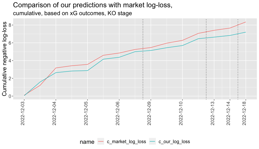
Since we took the group game odds directly from the market, our model was not really applied to these matches. Nevertheless it might be interesting to see how we performed. Effectively this is a test of pre-tournament against pre-match odds. The two figures below present the cumulative and game-by-game log-loss comparisons.

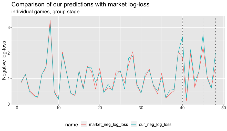
The performance tracks each other very closely with some divergence occuring towards the end of the group stage. This seems very natural. Betting odds capture the information available at the time and there is more relevant information that becomes available as more matches are observed.

One obvious version of new information would be that having seen each team play a couple of matches, we have a better sense of their tournament ability. But, in fact, there appears to be little effect from this. The divergence between pre-tournament and pre-match odds can be ascribed here to a single factor—asymmetrically dead rubbers.

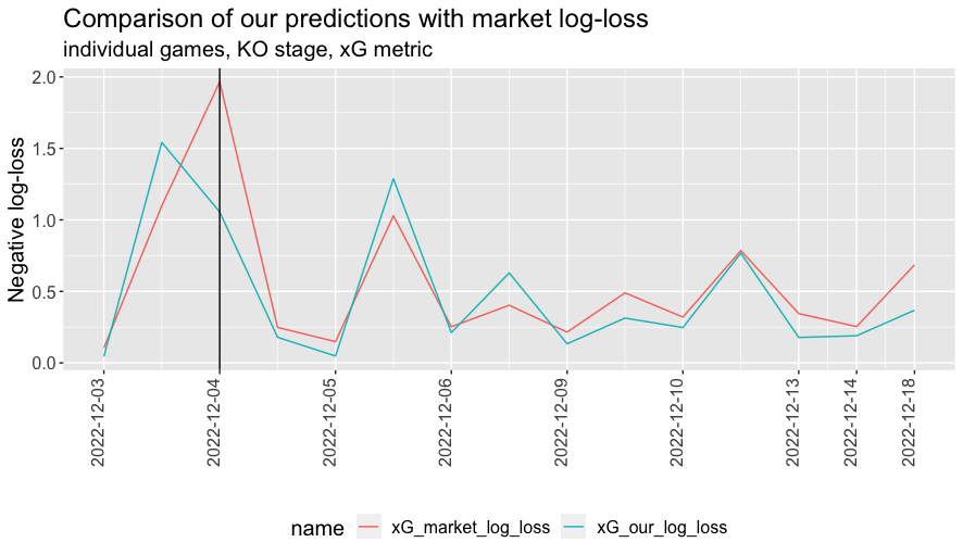
As can be seen below, the difference is explained by just three matches. They were Tunisia–France, Cameroon–Brazil, South Korea–Portugal, which all ended in upsets and are indicated by the dotted lines in the plot above.

These were precisely the matches where the favourite had already won both of their group matches so far and qualified for the next round, likely as group winners, before the final group match. We might then reasonably expect them to rest some of their key players and generally not be so motivated. On the other hand, the other team were super-motivated both by the possibility of a qualifying spot and of being able to topple a favourite and thus take something positive from the World Cup. The immediate pre-match odds took account of this when compared to the pre-tournament odds.

Knock-out stage

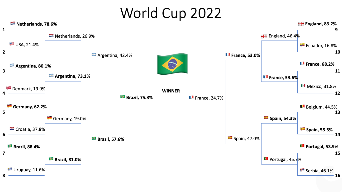
Turning to the more interesting part, how did we do on the knock-out stage matches? As a reminder, our initial predictions for the knock-out stage that we made in our original blog post are shown below (based on running 10,000 simulations of the World Cup with the probabilities determined by our model).

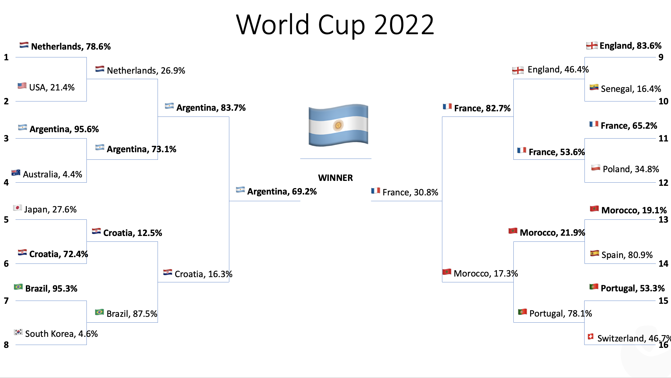
For comparison, we also present the actual outcomes of the knock-out stage together with the probabilities our model assigned to them.

The overall performance of our model in terms of cumulative log-loss is summarised in the plot below. Dotted lines mark the end of the Round of 16, quarter-finals and semi-finals respectively.

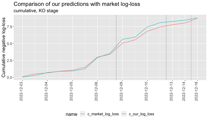
Coming into the quarter-final weekend we felt pretty good; we had correctly predicted six of the eight quarter-finalists and six of the eight group winners. In the round of sixteen, we correctly predicted seven of the eight match outcomes, with the one we got wrong being Morocco’s victory over Spain on penalties. This is a notable success compared to other attention-grabbing predictions.

Then, as the plot above shows, it began to unravel a little with the victories of Morocco over Portugal and Croatia over Brazil. But then we made some ground back in the semi-finals and even more with Argentina’s victory over France in the final.

In the end the market odds bested us by just 0.04. The median of our absolute match-level log-loss differences in the KO-stage was 0.16, so it seems not unfair to claim 0.04 as noise, and that our model based solely on pre-tournament data matched the performance of pre-match odds in prediction terms.

An alternative metric

That is a decent result given how much more information those pre-match odds included compared to our pre-tournament data. But we’re not content with a draw; we think we (might) deserve the win on this one.

One of the joys of football is the propensity for upsets. One of the authors of this post knows this well as a Coventry City fan. Two years after winning the FA Cup in 1987 (in probably the greatest ever FA Cup final match - there will never be a goal quite like Keith Houchen’s diving header), Coventry, at the time in fifth place in the top league of English football, went on to lose to Sutton United, a non-league team languishing in 13th place in the Vauxhall conference, 100 places below them. These events, while rare enough to be intriguing, are more common in football than in other high-profile sports.

High-scoring sports such as rugby union, basketball or cricket, exercise a type of score Central Limit Theorem where a lesser-favoured team may be able to score and even win portions of a game but over the entire match the aggregate scoring ability will tend towards the mean with a reduced variance. In contrast, football matches often have only a few goals. The randomness of the form of a striker or goalkeeper on a particular day or the bounce of the ball can therefore have a larger impact. Over many matches these more arbitrary elements will balance out, so that shocks over a league season are much rarer (though Leicester!).

This might suggest that there could be a better measure for a match than goals, in the sense that it would be more reflective of a team’s performance and would be a better predictor of future performance. This is indeed one of the claims made for the expected goals (xG) metric.

If we are prepared to believe this, and there seems to be some evidence for the claim, then it would be reasonable to measure predictions against the xG outcome of a match i.e. where the winner is the team that achieved the highest xG, since this is a better reflection of actual performance, stripped of the arbitrariness of goals.

For this purpose we take our xG outcomes from @xGPhilosophy on Twitter. If we re-run the log-loss measure with outcomes based on xG, what do we find? We win, and clearly! We beat the market by 1.15, with the median absolute match-level log-loss difference now being 0.10.

We suspect that a number of readers at this point might be a bit sceptical. You buy the argument about goals being a bit arbitrary, but some of the things that contribute towards the difference between xG and goals—striker or goalkeeper proficiency, for example—are important parts of the game.

Sceptics might also reasonably point out that our xG outperformance would be wiped out with the reversal of a single match: Poland-France, which Poland won 1.81-1.22 on xG, but France won 3-1 in reality (solid vertical line in the plot above). On the other hand, the argument that xG is more predictive of future performance seems quite persuasive, and this is the only one of the fifteen matches that could have reversed the finding with some other match reversals working in our favour.

Overall, we share the concerns, and wouldn’t claim that xG is the right way to look at it and goals the wrong way, but rather that they both have merit and given we drew on goals and won on xG, it would seem that there might be something being captured in our crude model that is working.

Ultimately, if the claim that xG is a better long-term predictor than goals is correct, and our outperformance based on xG is meaningful, then if you examined enough tournaments you would expect our method to work based on goals too. We have only analysed two tournaments, so can’t really comment on this, but they do not contradict the claim.

Let’s talk about money

Before speculating on what it might be that causes the model to work, it is worth addressing the measure used here. Log-loss is a reasonable way to measure predictions, but is more of academic interest (meant literally and perjoratively).

In the real world, when looking at betting odds, people care more about whether they can make money.

In order to turn predictions into money one needs a betting scheme, a method by which one turns those predictions into bets. Then, one can then measure the success of predictions by the profit or loss they generate under the betting scheme.

A good place to start with a betting scheme is to consider the expected return from a bet, given your predictions. In the knock-out stage matches, we were predicting the probability of reaching the next round i.e. it was a binary outcome, either Team 1 progressed or Team 2. If $p_i$ is the probability that Team $i$ progresses then $p_2 = 1 - p_1$. Our expected return in pounds from betting £1 on Team $i$ is then,

$$ \mathbb{E}[\text{return}]=p_i (o_i - 1) - (1-p_i) = p_io_i - 1, $$

where $o_i$ are the European odds for Team $i$ winning.¹ For each match, we can calculate the expected return from backing either Team 1 or Team 2 in this way. Note that there may not be a positive expected-return bet from backing either team if the market is sufficiently wide and our predictions are sufficiently well-calibrated to the market.²

A typical betting scheme would be to bet an amount, £1 say, whenever the expected return is above a specified threshold. One might argue that this threshold should be zero—you should bet whenever you think you are going to win—but often people are a bit more cautious. Models have noise and you want to identify the real opportunities.

Also betting has operational costs, the time taken to post money with bookmakers and make the bet. So often this threshold is set above zero (see, for example, this paper, which is very much in the spirit of our model, in using market odds as its data, and effectively takes a threshold of approximately 5%).

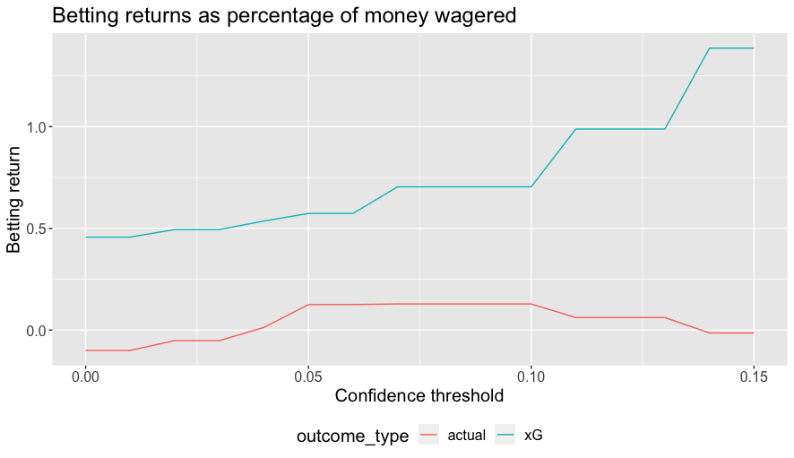
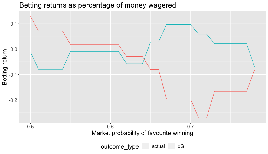
The figure below shows the return, calculated as net return divided by total money wagered for different thresholds, based on both goals and xG outcomes for confidence thresholds for which at least five bets would have been placed³.

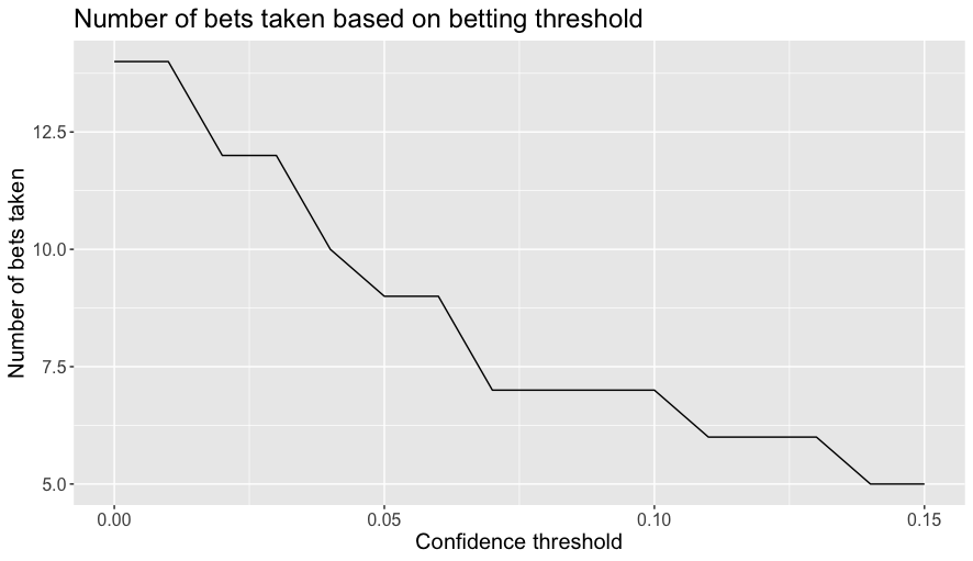
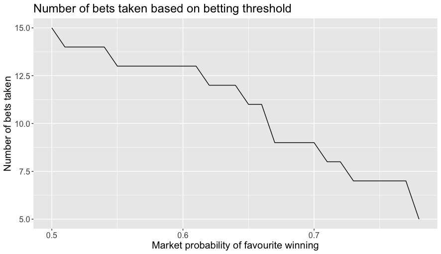
The next plot show the number of bets placed as a function of the confidence threshold.

Using xG is even more tenuous here—good luck finding a bookie who will pay out based on xG—but if the argument is correct that xG is a better future predictor of outcomes then it may give a better indicator of expected performance of the betting scheme. The maximum possible return from this strategy for actual outcomes is 12.9% of the capital wagered, which is realized when using a confidence threshold between 0.07 and 0.1.

While picking a threshold somewhere in the range between, say, 0.05 and 0.1 might have made for a reasonable heuristic, these optimal betting returns are obviously based on hindsight.

Another more serious concern is that while there look to be some tempting returns here, we have by this point travelled well-down Gelman’s garden of forking paths and based our argument on very little data, even more so when the betting scheme filters so we are only looking at a handful of matches.

Why does the model work?

Whichever way you cut the data and admitting it’s limitations given just the fifteen data points, the model does seem to work well against pre-match odds, which begs the question “why?”

Often when doing data analysis one finds a pattern and is interested in determining whether it is real or just a happenstance of the data. One natural consideration is whether there are good substantive reasons for why the pattern would exist.

In our case, we seem to have found that a crude model based on much less information can perform comparably with, perhaps even better than, the wisdom of the market. What could account for such a phenomenon?

In our last post, we discussed how our model had the effect of extremising the strength of teams, so that, for example, the probability of winning the tournament was increased for the strongest teams and decreased for weaker ones when compared to betting market odds as shown in plot below.

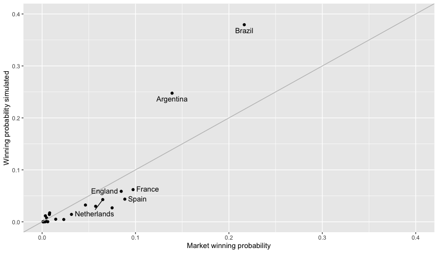
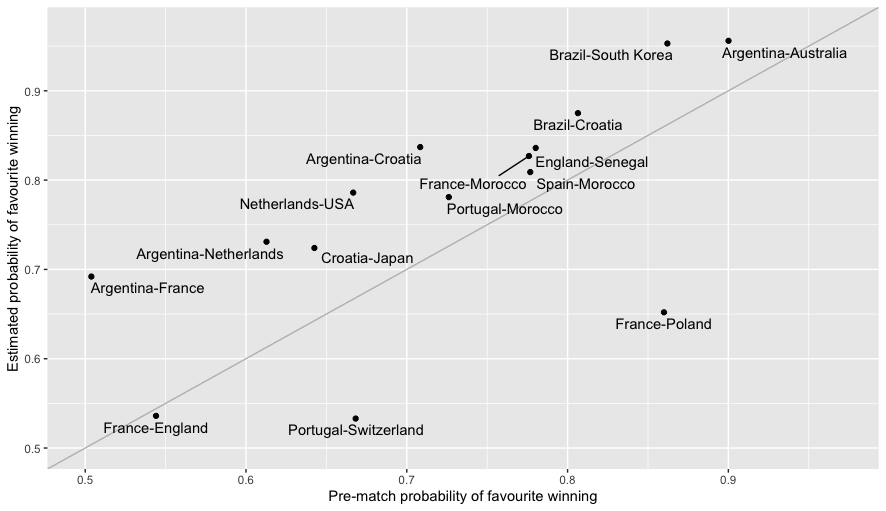
For the purpose of predicting individual matches, this meant that in most cases the estimated probability of a favourite winning was greater under our model than under the market odds, see the next plot.

The most obvious explanation then would be the so-called “favourite-longshot bias” (FLB), for which there is an academic literature stretching back decades. Somewhat confusingly the term ``favourite-longshot bias" seems to be applied both to situations where backing favourites produces better returns than from backing long-shots and the exact opposite.

As a group of cyncical statisticians, we can’t help sniffing the whiff of publication bias. On the other hand, this recent review article suggests that the findings for situations like ours, where there are two competitors and there is a binary outcome, are more consistently for better returns from backing a favourite. It offers a number of possible reasons, as do other well-cited articles here and here.

Perhaps the most appealing explanations recognise that the activity of betting, and therefore the betting market, is not driven solely by a rational evaluation of the chances of different teams.

The figure below shows the results of a betting scheme where we back the favourite if the betting market implied probability of it winning are greater than a certain percentage. It seems not especially persuasive for a favourite-based betting scheme, and not at all similar to the betting outcomes observed under our model, so it doesn’t seem like a very satisfactory explanation for the success of the model, such as it is.

The next plot shows the number of bets placed when backing the favourite as function of the market implied winning probability.

In conclusion, we’re not really sure what to make of this. Any conclusions based on so few matches, especially when filtered in the betting schemes, are likely to be unreliable at best. But the results we got here are consistent with what we saw at Euro 2020, so we still think there might be something to the method. We look forward to wheeling it out again at Euro 2024 and exploring some updated methods and analysis.