Tea & Stats

Sports prediction has exploded in the last couple of decades with entire journals, conferences and books devoted to it.

Much of this focuses on utilising ever-greater amounts of data, with soccer, for example, now providing sub-second ball and player tracking data.

But sometimes it is nice to try to do more with less.

Here we (Ian Hamilton, Stefan Stein and David Selby) describe a method that we applied to predict the results (indeed all possible match outcomes) of the Euro 2020 football tournament, that took just 120 data points and two linear regressions, yet managed to beat the market over the course of the tournament (based on the accumulated log-loss of match outcomes against predictions taken from the market odds immediately prior to the match).

All data analysts know the well-worn phrase: “garbage in, garbage out”. The corollary to this though is that when you have good data then it is easier to make good inferences. When one is considering predictions, what data would one most want?

One great form of data would be to have the predictions of a bunch of sophisticated data analysts and to be able to take some kind of conviction-weighted poll of those predictions. Fortunately (at least in some economists' imaginations) that is exactly what a market provides (we’re not entirely convinced by this, a point to which we will return). Betting markets on major tournaments are highly liquid and their prices readily accessible. They therefore provide excellent data for us to work from. But our aim here is to predict the outcome of all possible matches including those that might occur in the later rounds based on what we know pre-tournament.

There are, of course, no available odds to those KO matches pre-tournament because no-one knows what they will be. So how can we use what we do know to construct those probabilities?

We begin by taking a foundational model in Sports statistics (and the model that formed the basis of the PhDs of two of the authors of this blog post). First described by Ernst Zermelo in 1929, he made the crucial error of publishing the relevant article in German, allowing two upstart Americans to nab the glory nearly a quarter of a century later and have the model named after them. Thus it is known now as the Bradley–Terry model. It expresses the probability that a team $i$ beats a team $j$ as $$ p_{ij} = \frac{\pi_i}{\pi_i + \pi_j}, $$ where $\pi_i$ is the ‘strength’ of $i$. It can also be represented as a generalised linear model $$ \text{logit}(p_{ij}) = \lambda_i - \lambda_j, $$ where $\lambda_i = \log (\pi_i)$.

The Bradley–Terry model has some appealing statistical features, such as being the unique model for which the number of wins for each team is a sufficient statistic for the strength parameters (consistent with round robin ranking), and being the entropy and likelihood maximising model subject to the (highly plausible) constraint that the expected number of wins for a team given the matches observed is equal to the actual wins observed. As Stob (1984) put it, “What sort of a claim is it that a team solely on the basis of the results should have expected to win more games than they did?” This might be seen as failing to appreciate the bias present from finite observations. Nevertheless, it reflects the intuitive appeal of the condition.

Typically the Bradley–Terry model is applied to a set of results, for the purpose of prediction or ranking. Strength parameters can be estimated for each team by maximum likelihood estimation, using the likelihood function $$ L(\boldsymbol{\lambda}) = \prod_{i<j}\binom{m_{ij}}{c_{ij}}p_{ij}^{c_{ij}}(1-p_{ij})^{m_{ij}-c_{ij}}, $$ where $c_{ij}$ is the number of times $i$ beats $j$ and $m_{ij}= c_{ij}+c_{ji}$ is the number of matches between $i$ and $j$.

We could apply that method here based on historic performances, but:

1. there are not enough recent useful results to estimate strengths reliably;
2. market prices are likely to be more informative;
3. this doesn’t account for draws.

Addressing the last of these first, the model was extended to account for draws by Davidson (1970), and later by David Firth to take account of the standard football point scheme of three for a win, one for a draw, to give, $$ \mathbb{P}(i \text{ beats } j) = \frac{\pi_i}{\pi_i + \pi_j + \nu(\pi_i \pi_j)^{\frac{1}{3}}}, $$ $$ \mathbb{P}(i \text{ draws with } j) = \frac{\nu(\pi_i \pi_j)^{\frac{1}{3}}}{\pi_i + \pi_j + \nu(\pi_i \pi_j)^{\frac{1}{3}}}. $$

Note that even with draws, $$ \frac{p_{ij}}{p_{ji}} = \frac{\pi_i}{\pi_j} \quad \text{ or } \quad \text{logit}(p_{ij})= \lambda_i - \lambda_j. $$

In the present situation, we can estimate the intra-group log-strengths $r_i=\log s_i$ by linear regression: $$ \log \left(\frac{p_{ij}}{p_{ji}}\right) = r_i - r_j, $$ since $p_{ij}$ are known from market odds.

So now we have an estimate for the strength of a team relative to other teams in its group, but to be able to predict any possible match we need to know the strength of a team relative to all other teams. In order to do this, we make some assumptions:

1. Team $i$’s overall strength $\pi_i$ is a scaling of its intra-group strength $s_i$ by a factor dependent on its group $\gamma_{G(i)}$ $$ \pi_i = \gamma_{G(i)} s_i \quad \text{ or equivalently } \quad \lambda_i = \log\gamma_{G(i)} + r_i $$
2. The strength of every team’s unknown final opponent is the same $$ p_{io} = \mathbb{P}(i \text{ winning tournament} \mid i \text{ reaches final}) = \frac{\pi_i}{\pi_i + \pi_o}, $$ where $\pi_o$ is the strength of the unknown final opponent.

We can calculate $p_{io}$ from market odds since $$ p_{io} = \frac{\mathbb{P}(i \text{ winning tournament})}{\mathbb{P}(i \text{ reaches final})} $$ and both these odds — outright winner and reaching the final — are available pre-tournament. Then we have that $$ \log \left(\frac{p_{io}}{p_{oi}}\right) = \lambda_i - \lambda_o = \log\gamma_{G(i)} + r_i - \lambda_o, $$ and we can estimate $\log\gamma_{G(i)}$ and $\lambda_o$ through linear regression.

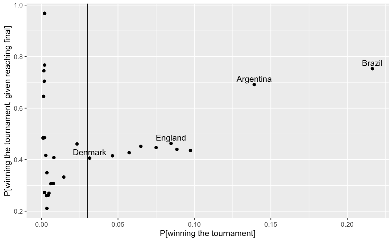
One thing to look out for here is that some of these odds are very large and not well-calibrated. For example, according to oddschecker.com the odds of Qatar winning the tournament are 500/1 and the odds of them reaching the final are 500/1, so conditional on them reaching the final the market says they have a 100% chance of winning! This is clearly nonsense, and is due to the fact that for the more unlikely winning teams, these odds are not well-calibrated and so should be discarded. Exactly which ones to discard is a matter of judgement. For Euro 2022 we arbitrarily excluded teams where the outright win odds were greater than 100/1.

For the World Cup we graphed $\log \left(\mathbb{P} \left[i \text{ winning tournament} \mid i \text{ reaches final} \right] \right)$ against $\log\left (\mathbb{P}\left[i \text{ winning tournament}\right] \right)$ and excluded at the point where a consistent relationship seemed to start to break down. For the World Cup we have included up to and including Denmark, the tenth ranked team, with a probability of winning the tournament of 30/1.

Now we can calculate the strengths of each team $$ \pi_i = \gamma_{G(i)} s_i, $$ and apply these through the Bradley-Terry model to predict the KO match results by applying $$ p_{ij} = \frac{\pi_i}{\pi_i + \pi_j}. $$

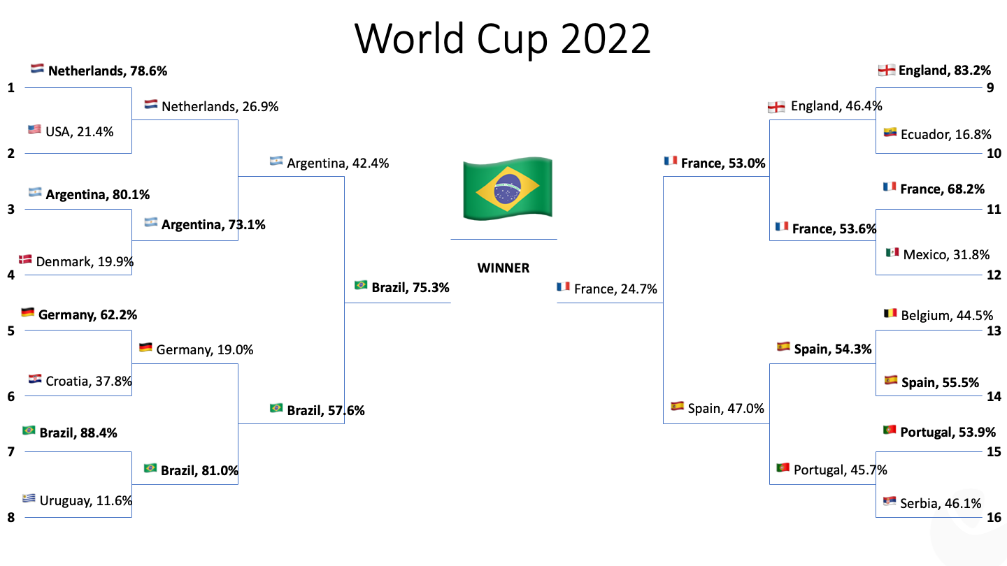
Using this method, we have determined a strength parameter for each team that can then be used to simulate the outcome of each match. We were keen to produce a route-to-the-final map, like the one in the presentation that inspired us to write this post (well worth a watch).

To get a better idea of how these probabilities play out, we simulated 10,000 runs of the World Cup with them. Here are the empirical probabilities of winning the tournament. Our method only gives match outcomes (win, lose, draw), so where teams were tied on points in a group, we used a procedure whereby with 50% probability the tied teams were ranked in order of their strength parameters and with 50% probability they were ranked randomly.

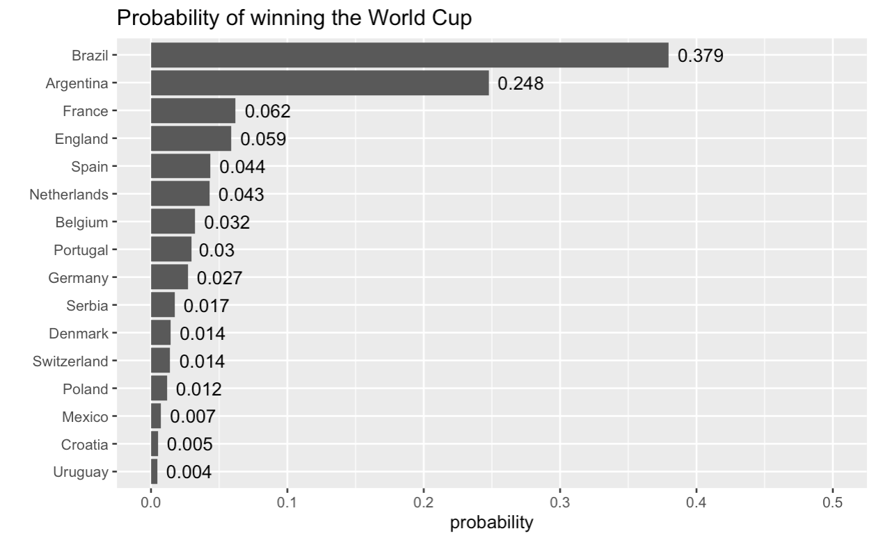
Brazil is clearly the favourite with a 37.9% chance of taking home the Cup, followed by Argentina, with a 24.8% chance Both of them are far ahead of the third-ranked (France, 6.2%) and fourth-ranked (England, 5.8%) teams.

Looking at the results of the simulation runs, we also extracted the “dominant path” most likely to lead to Brazil’s victory. Without further ado, here are our headline predictions:

As with any model, there are limitations. It is obviously (and unapologetically) a bit crude. For example, we are calibrating the strengths based on data for the 90-minute match results and applying them to the outcomes of KO matches, potentially after extra-time or penalties for example. We are also trusting betting odds to represent neutral value with the marginal price-maker being an informed individual, but betting is often a pursuit of the heart as much as the head and the notably different betting proclivity in different countries might suggest that some teams odds are likely to be skewed by this more than others.

But given these limitations, it is perhaps remarkable that when applied to Euro 2020 it outperformed the market (if taking the odds immediately prior to each match). Three possible explanations are:

1. betting markets overweight in-tournament performance in their odds creation. In most football prediction, analysts have huge amounts of data off which to work with clubs playing dozens of competitive matches each season. In the international arena, teams play fewer matches against opposition of more varied quality and in more varied situations of competitiveness (qualifying matches vs friendlies vs tournament etc.), so perhaps their methods are not so well-calibrated to this sparser data scenario;
2. the equal strength final opposition assumption is a strong one that boosts the probability of well-favoured teams winning, and it happened to be that well-favoured teams did well in Euro 2020;
3. England’s (surprising?) run to the final meant that the pre-tournament odds that (perhaps) featured a lot of heart-based backing (in possibly the biggest sports betting market in Europe) were supportive of the success of our scheme.

We would be inclined to think that some combination of the last two of these explanations are most likely, but another piece of evidence comes from other predictions for that tournament.

Our prediction work was done as part of the RSS Euro 2020 prediction competition. We came second, but the winner had a completely different method based on previous match outcomes and produced very similar performance to us, also beating the market, with the same being true of the third-placed entrant, who took a different approach again.

It’s possible that all our approaches overly-favoured favourites and that was how we came to be ranked highest. Alternatively, perhaps markets do over-react to in-tournament performance compared to pre-tournament assessments.

For more information and the full table of outcome predictions, check out the GitHub repository.