Tea & Stats

As part of my first foray into data science, I decided to have a go at opinion mining on Twitter. It’s common knowledge that everything stops for tea, but how much does the Twittersphere agree? And what else are microbloggers saying about the drink?

Using the free R statistical software it is very easy to start data mining on Twitter¹. A short R script quickly retrieved 699 recent tweets containing the tag #tea. The code looks something like this:

library(twitteR)
cred <- OAuthFactory$new(...)
...
load("twitter authentication.Rdata")
registerTwitterOAuth(cred)
require(plyr)
data<- searchTwitter("#tea", n=1500, cainfo="cacert.pem")
text = laply(data, function(t) t$getText())

Before anything interesting can be gleaned from the dataset, some housework must be done. Text mining² removes irrelevant URLs, punctuation, symbols and “stop words”, leaving each tweet ready for scrutiny.

So what are our friends on Twitter saying about tea? Finding out calls for a graph. But not just any graph: a word cloud³, displaying words according to frequency.

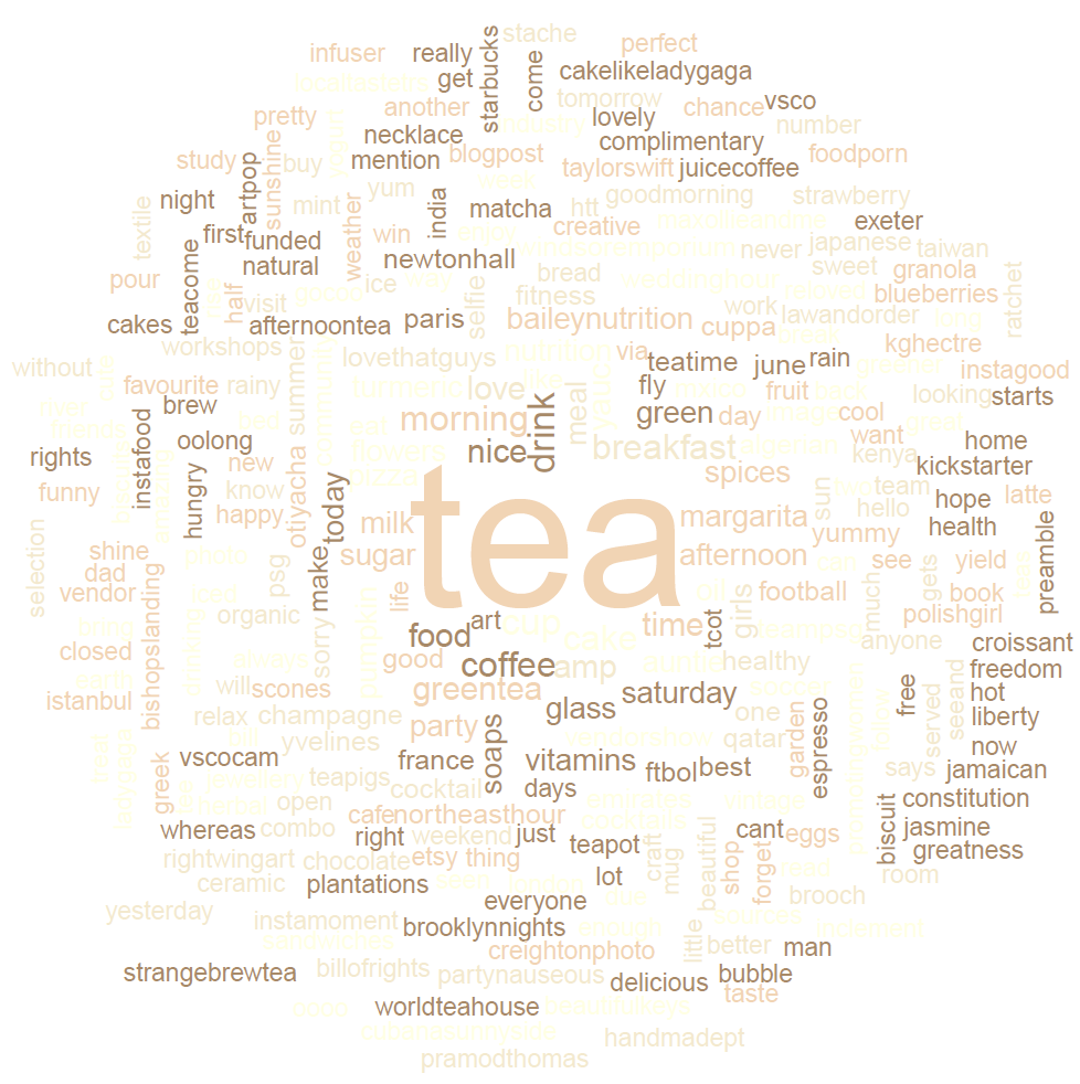
Obviously every tweet contains “tea” because that’s what was sought. People also like to discuss milk and sugar, as well as coffee (possibly during cataclysmic breakfast drink dilemmas). To the right of centre, tcot stands for “top conservatives on Twitter”, who enjoy talking about tea — and tea parties — as much as anyone. Other notable phrases include “freedom”, “greatness”, “best” and “delicious”. But we’ll do some more objective analysis shortly.

For variety, I also had a go at mining Twitter’s public streaming API for a larger sample, this time using Python. Here’s what some ten thousand tweets say about Canadian pop star Justin Bieber:

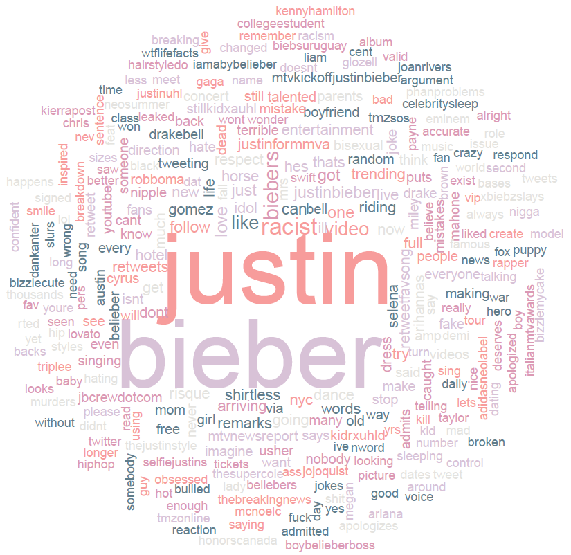
He’s racist? And shirtless. Who knew?

To assess public opinion more objectively, we can perform sentiment analysis, which involves assigning a mood to each tweet and observing the distribution⁴. A tweet’s mood score derives from comparing each constituent word against a database of “positive” and “negative” English words then adding and subtracting 1 respectively. A total less than -2 is very negative, zero is neutral and greater than +2 is very positive.

For example, this tweet gets a score of +5:

@justinbieber i’m so happy to say : “Justin Bieber is my idol and he’s perfect” because i love you so much you’re a very good man

whereas this one is assigned a score of -4:

Justin Bieber has serious issues, i wish he’d just sort his shit out because I for one am sick of seeing stupid crap about him in the news

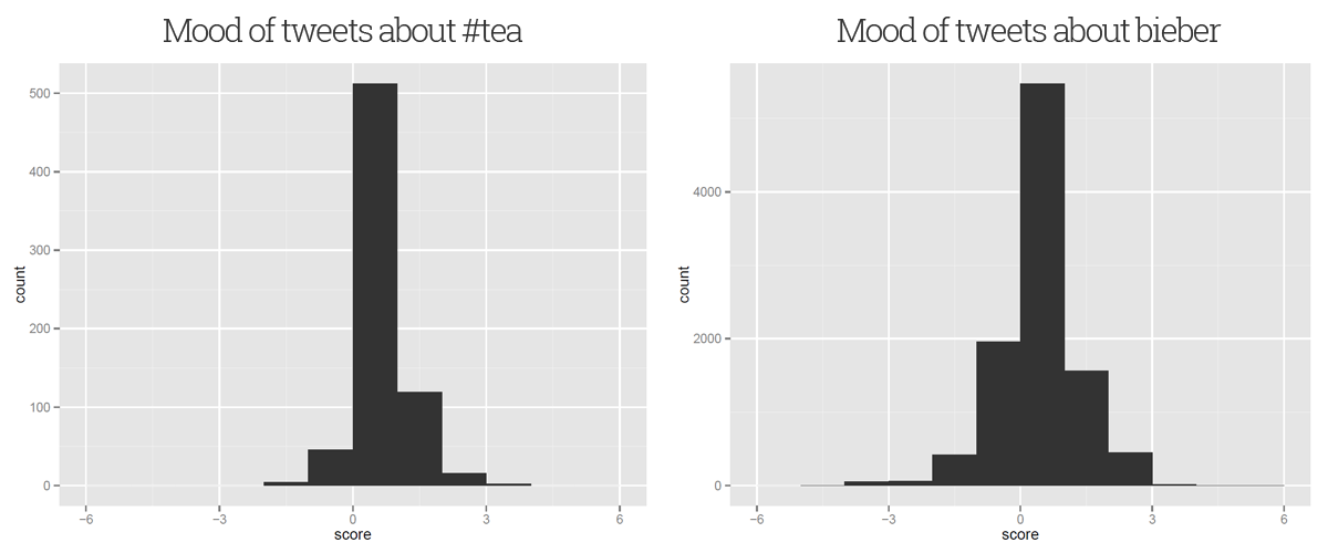
Our #tea dataset has a score distribution that’s mostly positive, with a mean sentiment score of +0.15 and a variance of 0.36. Clearly our intuition is correct and people really do like tea. Indeed, nobody really had much of a bad word to say about the beverage; the minimum score given was -2, which could easily have been obtained from a false-negative tweet like “I hate people who dislike #tea” (though it wasn’t).

On the other hand, the outlook isn’t so rosy for our friend Justin. From our dataset of 10,003 tweets, the mean mood score is -0.07, which is slightly negative. He’s a divisive topic of discussion, too: the score variance is 0.87, giving a more widely-spread distribution of sentiments.

So it’s official. Twitter likes tea more than it likes Justin Bieber. Probably. Time for a cuppa.