Tea & Stats

Logistic regression

What’s a logistic regression model? Suppose we want to build a machine that classifies objects in two groups, for example ‘hot dog’ and ‘not hot dog’. We will say \(Y_i = 1\) if object i is a hot dog, and \(Y_i = 0\) otherwise.

A logistic regression model estimates these odds, \[ \operatorname{odds}(Y = 1) = \frac{\operatorname P(Y = 1)} {\operatorname P(Y = 0)} = \frac{\operatorname P(Y = 1)} {\operatorname 1 - \operatorname P(Y = 1)} \] and for mathematical and computational reasons we take the natural logarithm of the same—the log odds. As a generalised linear model, the response (the log odds) is a linear combination of the parameters and the covariates, \[\operatorname{log-odds}(Y = 1) = X \beta,\] where \(X\) is the design matrix and \(\beta\) is a vector of parameters to be found.

Classical statistical inference involves looking for a parameter estimate, \(\hat\beta\), that maximises the likelihood of the observations given the parameters. For our hot dog classification problem, the likelihood function is \[\mathcal{L} = \prod_i \operatorname P(Y_i=1)^{y_i} \operatorname P(Y_i = 0)^{1 - y_i}\] or, taking logs, \[\log \mathcal{L} = \sum_i \Bigl[ y_i \log \operatorname P(Y_i = 1) + (1-y_i) \log \operatorname P(Y_i = 0) \Bigr]. \]

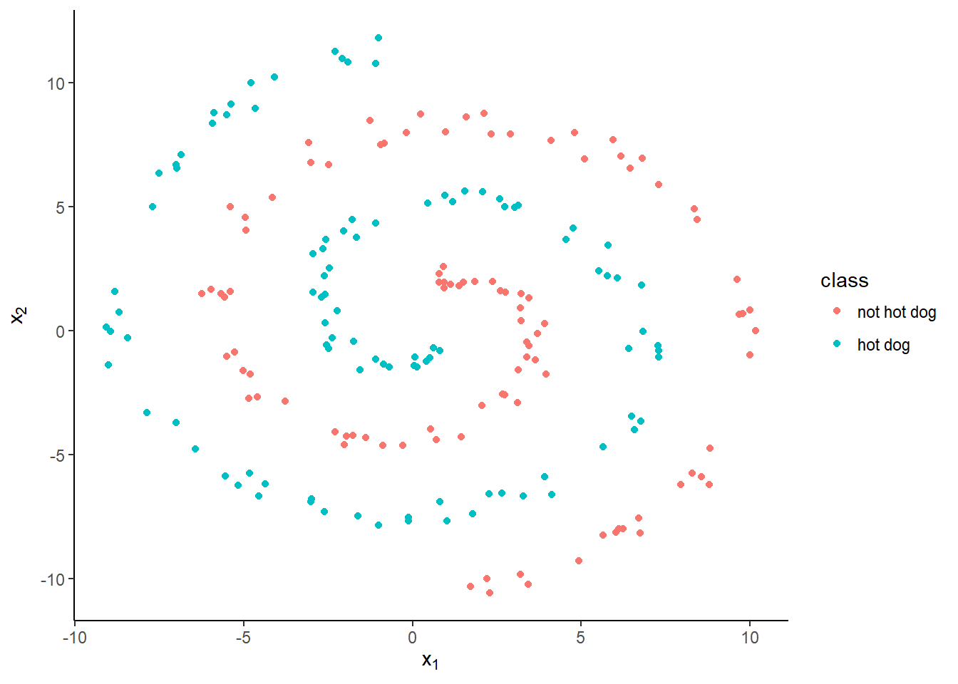
Let’s imagine we have been given some two-dimensional data about a sample of objects, along with their labels. Our sample data set includes 200 observations. Here is a random sample of five:

x1	x2	class
8.81	-6.19	not hot dog
10.00	0.84	not hot dog
-1.78	4.48	hot dog
6.83	-0.02	hot dog
1.71	-10.29	not hot dog

And a scatter plot of all of them:

Fitting a logistic regression model in R is easy:

logreg <- glm(class ~ x1 + x2, family = binomial, data = hotdogs)

But as the decision boundary can only be linear, it doesn’t work too well at distinguishing our two classes. Logistic regression classifies 134 (67%) of our objects correctly.

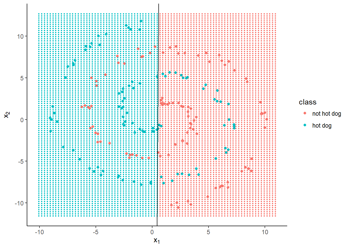
Nonlinearity is where neural networks are useful.

Artificial neural networks

An artificial neural network is so called because once upon a time it was thought to be a good model for how neurons in the brain work. Apparently it isn’t, but the name has stuck.

Suppose we have some inputs, \(\mathbf x\), and known outputs \(\mathbf y\). Then the aim of the game is to find a way of estimating \(\mathbf y\) based on \(\mathbf x\). In a way, then, a neural network is like any other regression or classification model.

Neural networks (for classification, at least) are also known as multi-layer perceptrons. Like ogres and onions, they have layers—three to be exact.

The output layer is our estimate of the probability that objects belong to each class. The input layer comprises the covariates and an intercept, as before. In the middle, there is a hidden layer, which is a transformation of the input space into \(h\) dimensions, where \(h\) is a number chosen by us. We then perform a logistic regression on this transformed space to estimate the classes.

It works like this.

1. Generate \(h\) different linear combinations of the input variables.
2. Apply an ‘activation’ function, that for each observation, turns each hidden node ‘on’ or ‘off’.
3. Fit a logistic regression model to these \(h\) transformed predictors, plus an intercept.
4. Adjust the parameters of both the input and the output to maximise likelihood.
5. Repeat, ad nauseum.

If \(h = 1\) then there is only one linear combination of the predictors, which is effectively the same thing as having no hidden layer at all, i.e. ordinary logistic regression.

So we run a kind of logistic regression model on the inputs to generate a transformation of the feature space, then once more to classify our actual objects. Each iteration of the fitting or ‘training’ process adjusts both the transformation and the regression parameters.

Hidden layers

The input layer is a design matrix, \(\mathbf X = \begin{bmatrix}\mathbf 1 & \mathbf x\end{bmatrix}\). The output layer is a vector of estimated probabilities, \(\hat {\mathbf y}\). So far, this is exactly like our logistic regression model above.

A neural network adds a hidden layer, which you might think of as an intermediate design matrix between the inputs and the outputs. Deep learning is just a neural network with multiple hidden layers.

If there are \(d\) input variables then there are \(d+1\) input nodes—one for each covariate, plus an intercept, or ‘bias’ (because computer scientists like having separate names for everything).

In general there are \(k-1\) output nodes, where \(k\) is the number of possible classes. The \(k^\text{th}\) node would be the same as ‘none of the above’, so it is redundant. In a binary classification problem like ours, there is just one output node, because \(\operatorname P(Y=0) = 1 - \operatorname P(Y=1)\).

There are \(h\) nodes in the hidden layer, plus an intercept. Each of these is a linear combination of the inputs, passed through an activation function. The intercept does not depend on the nodes in the previous layer¹.

The activation function is often (not always) chosen to be the sigmoid function, another name for the logistic function, \[\sigma(x) = \frac 1 {1 + e^{-x}},\] the inverse of the logit \[\operatorname{logit}(x) = \log \left( \frac{x}{1-x} \right).\] If \(x\) is a probability of an event, then \(\operatorname{logit}(x)\) is its log odds.

Forward propagation

Starting with the inputs, we feed forward through the network as follows.

Firstly, compute a linear combination of the covariates, using some weight matrix \(\mathbf W_\text{in} \in \mathbb R^{(d+1) \times h}\). \[ \mathbf z_1 = \mathbf{XW}_\text{in} = \begin{bmatrix}\mathbf 1 & \mathbf x\end{bmatrix} \mathbf W_\text{in} \] Next, apply an activation function to obtain the nodes in the hidden layer. The hidden layer \(\mathbf H\) might be thought of as a design matrix containing the output of a logistic regression classifying whether each node is ‘activated’ or not. \[\mathbf h = \sigma(\mathbf z_1)\] The intercept/bias is always activated, so it is fixed to be a vector of ones. \[\mathbf H = \begin{bmatrix} \mathbf 1 & \mathbf h \end{bmatrix} = \begin{bmatrix} \mathbf 1 & \sigma(\mathbf z_1) \end{bmatrix} = \begin{bmatrix} \mathbf 1 & \sigma(\mathbf {XW}_\text{in}) \end{bmatrix}\] For the output layer, compute a linear combination of the hidden variables, this time using another weight matrix, \(\mathbf{W}_\text{out} \in \mathbb R^{(h+1) \times (k-1)}\). \[\mathbf z_2 = \mathbf {HW}_\text{out} = \begin{bmatrix} \mathbf 1 & \mathbf h\end{bmatrix} \mathbf W_\text{out} \] Apply one more function to get the output \[\hat {\mathbf y} = \sigma (\mathbf z_2),\] which is a probability vector, \(\hat Y_i = \operatorname P(Y_i = 1)\).

Putting it all together, \[\hat {\mathbf y} = \sigma \left( \mathbf {H W} _ \text{out} \right) = \sigma \bigl( \begin{bmatrix} \mathbf 1 & \sigma ( \mathbf {X W} _ \text{in} ) \end{bmatrix} \mathbf W _ \text{out} \bigr).\]

It is straightforward to write a function to perform the forward propagation process in R. Just do

feedforward <- function(x, w1, w2) {
  z1 <- cbind(1, x) %*% w1
  h <- sigmoid(z1)
  z2 <- cbind(1, h) %*% w2
  list(output = sigmoid(z2), h = h)
}

where

sigmoid <- function(x) 1 / (1 + exp(-x))

Where do we get the weights from? On the first iteration, they can be random. Then we have to make them better.

Back propagation

So far we have been taking the parameters, or weights, \(\mathbf W_\text{in}\) and \(\mathbf W_\text{out}\), for granted.

Like parameters in a linear regression, we need to choose weights that make our model ‘better’ by some criterion. Neural network enthusiasts will say that we will train our multilayer perceptron by minimising the cross entropy loss. That’s a fancy way of saying we fit the model using maximum likelihood.

The log-likelihood for a binary classifier is \[\ell = \sum_i \Bigl( y_i \log \hat y_i + (1 - y_i) \log (1 - \hat y_i) \Bigr).\] We can maximise this via gradient descent, a general-purpose optimisation algorithm.

To minimise \(\ell = f(\mathbf W)\) via gradient descent, we iterate using the formula \[\mathbf W_{t+1} = \mathbf W_{t} - \gamma \cdot \nabla f(\mathbf W_{t}),\] where \(\mathbf W_t\) is the weight matrix at time \(t\), \(\nabla f\) is the gradient of \(f\) with respect to \(\mathbf W\) and \(\gamma\) is the ‘learning rate’.

Choose a learning rate too high and the algorithm will leap around like a dog chasing a squirrel, going straight past the optimum; choose one too low and it will take forever, making mountains out of molehills.

Using the chain rule, the gradient of the log-likehood with respect to the output weights is given by \[\frac {\partial\ell} {\partial \mathbf W_\text{out}} = \frac{\partial \ell}{\partial \hat {\mathbf y}} \frac{\partial \hat {\mathbf y} }{\partial \mathbf W_\text{out}}\] where \[\begin{aligned} \frac{\partial\ell}{\partial \hat{\mathbf y}} &= \frac{\mathbf y}{\hat{\mathbf y}} - \frac{1 - \mathbf y}{1 - \hat{\mathbf y}} = \frac{\hat{\mathbf y} - \mathbf y}{\hat{\mathbf y}(1 - \hat{\mathbf y})},\\ \frac{\partial\hat{\mathbf y}}{\partial \mathbf W_\text{out}} &= \mathbf{H}^T \sigma(\mathbf {HW}_\text{out})\bigl( 1 - \sigma(\mathbf{HW}_\text{out}) \bigr) \\ &= \mathbf H^T \hat {\mathbf y} (1 - \hat{\mathbf y}). \end{aligned}\]

And the gradient with respect to the input weights is \[ \frac {\partial\ell} {\partial \mathbf W_\text{in}} = \frac{\partial \ell}{\partial \hat {\mathbf y} } \frac{\partial \hat {\mathbf y} }{\partial \mathbf H} \frac{\partial \mathbf H}{\partial \mathbf W_\text{in}} \] where \[ \begin{aligned} \frac{\partial \hat{\mathbf y}}{\partial \mathbf H} &= \sigma(\mathbf{HW}_\text{out}) \bigl( 1 - \sigma(\mathbf{HW}_\text{out}) \bigr) \mathbf W_\text{out}^T \\ &= \hat{\mathbf y} (1 - \hat{\mathbf y}) \mathbf W_\text{out}^T, \\ \frac{\partial \mathbf H}{\partial \mathbf W_\text{in}} &= \mathbf X^T \begin{bmatrix} \mathbf 0 & \sigma(\mathbf{XW}_\text{in})\bigl( 1 - \sigma(\mathbf{XW}_\text{in}) \bigr) \end{bmatrix}. \end{aligned} \]

In the last step, we take for granted that the intercept column of \(\mathbf H\) doesn’t depend on \(\mathbf W_\text{in}\), but you could parametrise it differently (see footnotes).

A simple R implementation is as follows.

backpropagate <- function(x, y, y_hat, w1, w2, h, learn_rate) {
  dw2 <- t(cbind(1, h)) %*% (y_hat - y)
  dh  <- (y_hat - y) %*% t(w2[-1, , drop = FALSE])
  dw1 <- t(cbind(1, x)) %*% (h * (1 - h) * dh)
  
  w1 <- w1 - learn_rate * dw1
  w2 <- w2 - learn_rate * dw2
  
  list(w1 = w1, w2 = w2)
}

Training the network

Training is just a matter of initialising the weights, propagating forward to get an output estimate, then propagating the error backwards to update the weights towards a better solution. Then iteratively propagate forwards and backwards until the Earth has been swallowed by the Sun, or some other stopping criterion.

Here is a quick implementation using the functions defined above.

train <- function(x, y, hidden = 5, learn_rate = 1e-2, iterations = 1e4) {
  d <- ncol(x) + 1
  w1 <- matrix(rnorm(d * hidden), d, hidden)
  w2 <- as.matrix(rnorm(hidden + 1))
  for (i in 1:iterations) {
    ff <- feedforward(x, w1, w2)
    bp <- backpropagate(x, y,
                        y_hat = ff$output,
                        w1, w2,
                        h = ff$h,
                        learn_rate = learn_rate)
    w1 <- bp$w1; w2 <- bp$w2
  }
  list(output = ff$output, w1 = w1, w2 = w2)
}

Let’s train a neural network with five hidden nodes (like in Figure 1) on the hot dogs data.

x <- data.matrix(hotdogs[, c('x1', 'x2')])
y <- hotdogs$class == 'hot dog'
nnet5 <- train(x, y, hidden = 5, iterations = 1e5)

On my desktop PC, it takes about 12 seconds for the above code to run the 100,000 iterations. Not too bad for what sounds like a lot of runs, but what are the results like?

We can calculate how many objects it classified correctly:

mean((nnet5$output > .5) == y)

## [1] 0.76

That’s 76%, or 152 out of 200 objects in the right class.

Let’s draw a picture to see what the decision boundaries look like. To do that, we firstly make a grid of points around the input space:

grid <- expand.grid(x1 = seq(min(hotdogs$x1) - 1,
                             max(hotdogs$x1) + 1,
                             by = .25),
                    x2 = seq(min(hotdogs$x2) - 1,
                             max(hotdogs$x2) + 1,
                             by = .25))

Then feed these points forward through our trained neural network.

ff_grid <- feedforward(x = data.matrix(grid[, c('x1', 'x2')]),
                       w1 = nnet5$w1,
                       w2 = nnet5$w2)
grid$class <- factor((ff_grid$output > .5) * 1,
                     labels = levels(hotdogs$class))

Then, using ggplot2, we plot the predicted classes on a grid behind the observed points.

ggplot(hotdogs) + aes(x1, x2, colour = class) +
  geom_point(data = grid, size = .5) +
  geom_point() +
  labs(x = expression(x[1]), y = expression(x[2]))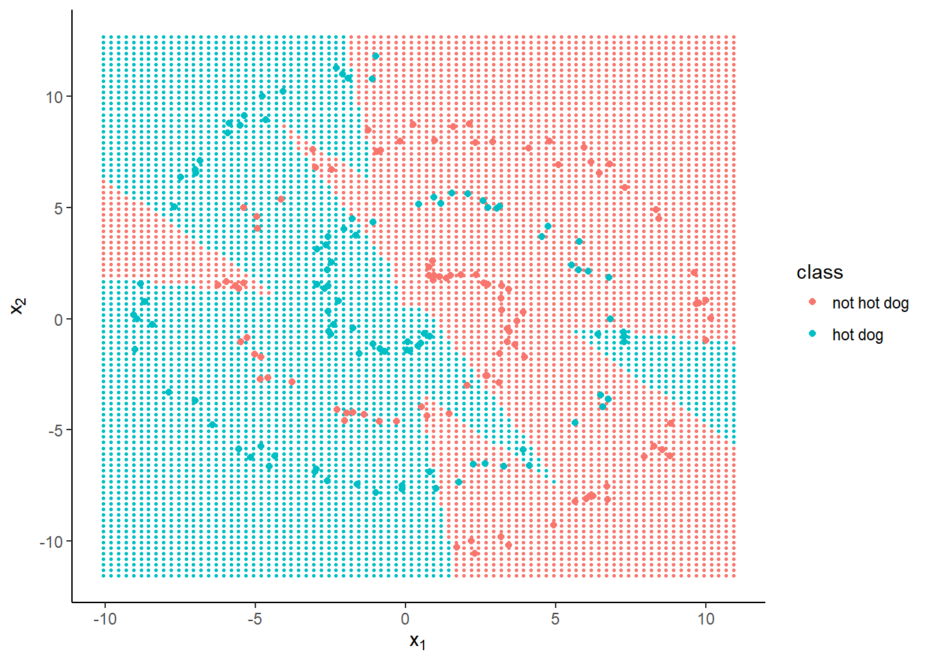

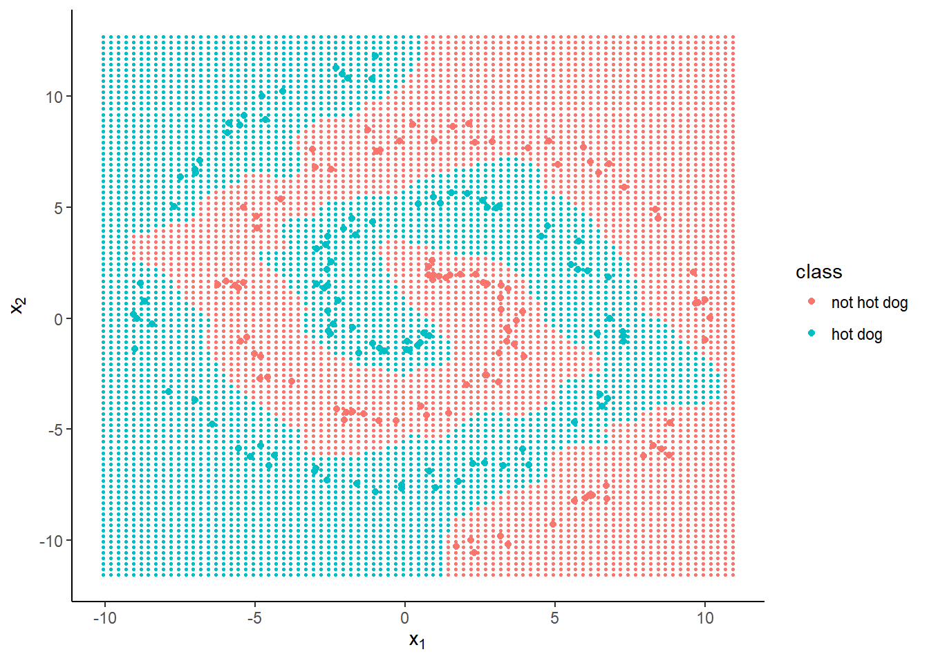
The regions the neural network has classified into ‘hot dog’ and ‘not hot dog’ can no longer be separated by a single straight line. The more nodes we add to the hidden layer, the more elaborate the decision boundaries can become, improving accuracy at the expense of computation time (as more weights must be calculated) and increased risk of over-fitting the data.

How about 30 nodes?

nnet30 <- train(x, y, hidden = 30, iterations = 1e5)

After 100,000 iterations, accuracy is 100%. The decision boundary looks much smoother:

And for completeness, let’s see what one hidden node (plus an intercept) gives us.

nnet1 <- train(x, y, hidden = 1, iterations = 1e5)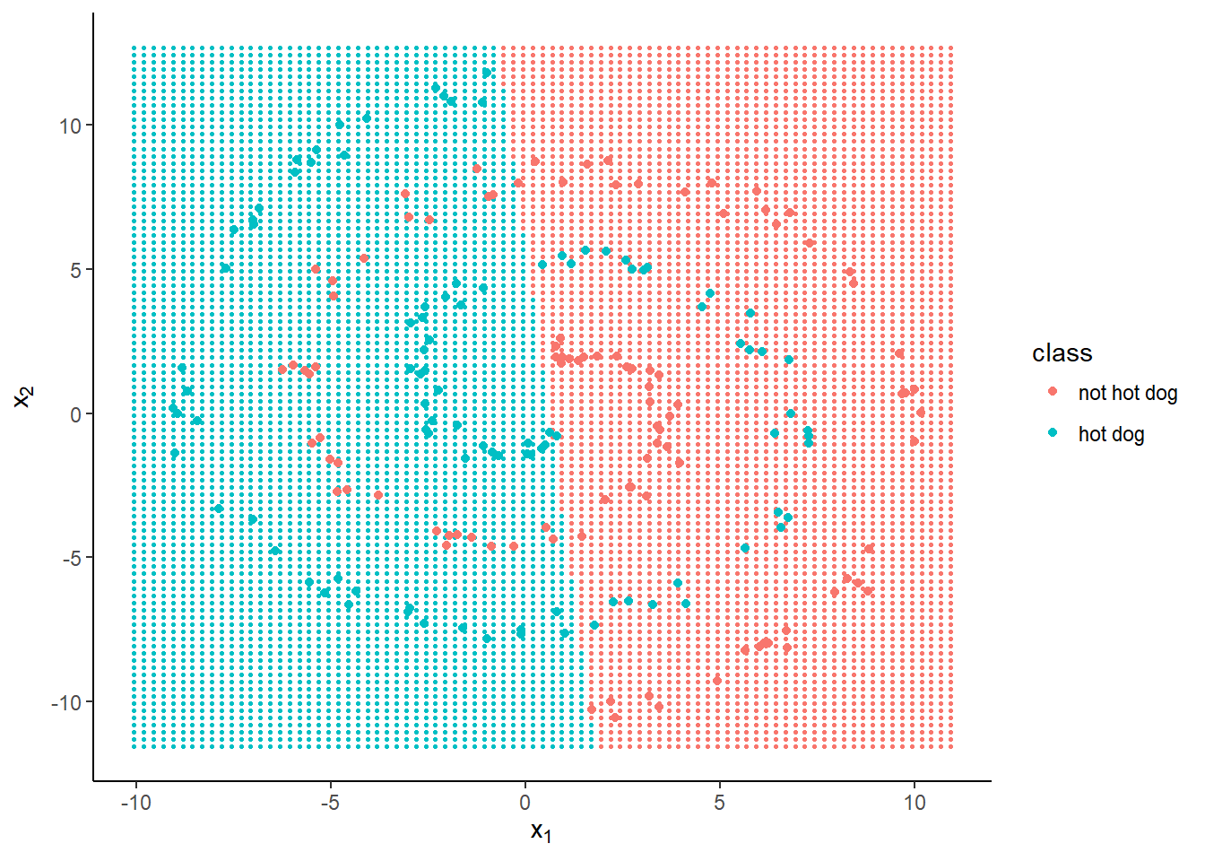

Much worse accuracy—68%—and the decision boundary looks linear.

R6 class implementation

The above code works, mathematically, but isn’t the most elegant solution from a user interface point of view. It’s a bit ad hoc. One of the annoying things about writing R functions is that, unless you use the global assignment operator (<<-) then the arguments are immutable.

Also, everything defined within the function scope is discarded. You can return the objects in a list, but this can be unwieldy and you have to extract each object one by one to pass into the arguments of the next function. And despite this we still have three functions and various objects cluttering the workspace.

Can we do better? A more flexible implementation is object orientated, using R6 classes.

The following class not only supports binary classification but also multinomial logistic regression, providing a high-level formula interface like that used when fitting an lm or glm with the stats package.

The maths for multi-class classification is very similar (partly thanks to the derivative of the softmax function—the multivariate generalisation of sigmoid—cancelling out in the gradient calculation) and most of the modifications are to do with wrangling R factors to and from indicator matrix representation.

library(R6)
NeuralNetwork <- R6Class("NeuralNetwork",
  public = list(
    X = NULL,  Y = NULL,
    W1 = NULL, W2 = NULL,
    output = NULL,
    initialize = function(formula, hidden, data = list()) {
      # Model and training data
      mod <- model.frame(formula, data = data)
      self$X <- model.matrix(attr(mod, 'terms'), data = mod)
      self$Y <- model.response(mod)
      
      # Dimensions
      D <- ncol(self$X) # input dimensions (+ bias)
      K <- length(unique(self$Y)) # number of classes
      H <- hidden # number of hidden nodes (- bias)
      
      # Initial weights and bias
      self$W1 <- .01 * matrix(rnorm(D * H), D, H)
      self$W2 <- .01 * matrix(rnorm((H + 1) * K), H + 1, K)
    },
    fit = function(data = self$X) {
      h <- self$sigmoid(data %*% self$W1)
      score <- cbind(1, h) %*% self$W2
      return(self$softmax(score))
    },
    feedforward = function(data = self$X) {
      self$output <- self$fit(data)
      invisible(self)
    },
    backpropagate = function(lr = 1e-2) {
      h <- self$sigmoid(self$X %*% self$W1)
      Yid <- match(self$Y, sort(unique(self$Y)))
      
      haty_y <- self$output - (col(self$output) == Yid) # E[y] - y
      dW2 <- t(cbind(1, h)) %*% haty_y
      
      dh <- haty_y %*% t(self$W2[-1, , drop = FALSE])
      dW1 <- t(self$X) %*% (self$dsigmoid(h) * dh)
      
      self$W1 <- self$W1 - lr * dW1
      self$W2 <- self$W2 - lr * dW2
      
      invisible(self)
    },
    predict = function(data = self$X) {
      probs <- self$fit(data)
      preds <- apply(probs, 1, which.max)
      levels(self$Y)[preds]
    },
    compute_loss = function(probs = self$output) {
      Yid <- match(self$Y, sort(unique(self$Y)))
      correct_logprobs <- -log(probs[cbind(seq_along(Yid), Yid)])
      sum(correct_logprobs)
    },
    train = function(iterations = 1e4,
                     learn_rate = 1e-2,
                     tolerance = .01,
                     trace = 100) {
      for (i in seq_len(iterations)) {
        self$feedforward()$backpropagate(learn_rate)
        if (trace > 0 && i %% trace == 0)
          message('Iteration ', i, '\tLoss ', self$compute_loss(),
                  '\tAccuracy ', self$accuracy())
        if (self$compute_loss() < tolerance) break
      }
      invisible(self)
    },
    accuracy = function() {
      predictions <- apply(self$output, 1, which.max)
      predictions <- levels(self$Y)[predictions]
      mean(predictions == self$Y)
    },
    sigmoid = function(x) 1 / (1 + exp(-x)),
    dsigmoid = function(x) x * (1 - x),
    softmax = function(x) exp(x) / rowSums(exp(x))
  )
)

What do each of the methods do?

• initialize is run every time you make a new network. It initialises the weight matrices to be the correct dimensions, populated with random initial values.
• fit runs one step of forward propagation but returns the result instead of storing it. Useful for predicting from new test data without changing the model.
• feedforward runs fit but saves the results, for training.
• backpropagate does what you might expect, saving the results for training.
• train runs forward and back propagation, storing the results and printing the progress to the console every trace iterations.
• predict uses argmax to estimate a single discrete class for each observation (whereas fit only returns probabilities).
• accuracy and compute_loss return the proportion of correct class assignments and the negative log likelihood (‘log loss’), respectively
• sigmoid, dsigmoid and softmax are utility functions.

Let’s see our fancy neural network in action on the famous iris data set. Firstly, initialise the network by specifying the input and output variables and the number of hidden nodes. (Let’s go for five.)

irisnet <- NeuralNetwork$new(Species ~ ., data = iris, hidden = 5)

I have implemented a formula interface so I can regress Species on the other four variables (Petal.Length, Petal.Width, Sepal.Length and Sepal.Width) without having to type it out in full.

That’s the framework assembled. Now we can train the model. No need to assign any new variables—the R6 object modifies itself in place.

irisnet$train(9999, trace = 1e3, learn_rate = .0001)
## Iteration 1000   Loss 151.054969487204   Accuracy 0.68
## Iteration 2000   Loss 81.6280605667542   Accuracy 0.853333333333333
## Iteration 3000   Loss 64.5735942975868   Accuracy 0.966666666666667
## Iteration 4000   Loss 51.0996158369837   Accuracy 0.973333333333333
## Iteration 5000   Loss 40.105949050699    Accuracy 0.973333333333333
## Iteration 6000   Loss 32.3280157122779   Accuracy 0.973333333333333
## Iteration 7000   Loss 27.0449301604686   Accuracy 0.98
## Iteration 8000   Loss 23.3961690114  Accuracy 0.98
## Iteration 9000   Loss 20.7875204792586   Accuracy 0.98

You might notice that the log loss is going down even while accuracy stays the same. This is because the model is becoming more or less confident about each of its predictions, even if the argmax doesn’t change.

Everything is stored inside the NeuralNetwork object.

irisnet

## <NeuralNetwork>
##   Public:
##     accuracy: function () 
##     backpropagate: function (lr = 0.01) 
##     clone: function (deep = FALSE) 
##     compute_loss: function (probs = self$output) 
##     dsigmoid: function (x) 
##     feedforward: function (data = self$X) 
##     fit: function (data = self$X) 
##     initialize: function (formula, hidden, data = list()) 
##     output: 0.968263186096496 0.962577356981835 0.965919909020745 0. ...
##     predict: function (data = self$X) 
##     sigmoid: function (x) 
##     softmax: function (x) 
##     train: function (iterations = 10000, learn_rate = 0.01, tolerance = 0.01, 
##     W1: 0.535763605328154 1.04640352732849 1.11188605221437 -1.7 ...
##     W2: -0.412354248171205 2.04939691705817 -1.70485310730503 -3 ...
##     X: 1 1 1 1 1 1 1 1 1 1 1 1 1 1 1 1 1 1 1 1 1 1 1 1 1 1 1 1  ...
##     Y: setosa setosa setosa setosa setosa setosa setosa setosa  ...

One other nice thing about R6 classes is you can chain methods together where they return self or invisible(self). So if I want to train for 1000 iterations and then predict for some new data, all in one line, it’s as simple as

irisnet$train(1000)$predict(newdata)

There are plenty of improvements we could make to the NeuralNetwork class but most of them are beyond the scope of this article, and left as an exercise to the interested reader. Here are some ideas:

• user-selectable activation functions, rather than hard-coded sigmoid
• regularisation, and including regularisation loss as part of compute_loss()
• arbitrary number of hidden layers, to enable deep learning (multiple hidden layers) or logistic regression (no hidden layer)
• regression as well as classification
• more intelligent initial weights
• changing learning rate over time

But you might be wondering: can I actually classify pictures of hot dogs with this? Probably not from raw pixels—image analysis is usually a job for a convolutional neural network, which is a more advanced topic for another day.

For further reading, try Chapter 6 of Deep Learning (2016) by Goodfellow, Bengio and Courville.

I hope you found this useful! Let me know if anything is unclear. Full source code for this post is available on GitHub.