Hello, R Markdown!
You’ll find this post in your _source directory. Unlike the other example post on this blog (found in _posts), this one was written in R Markdown.
This means you can generate plots:
plot(iris$Petal.Width, iris$Petal.Length,
     col = as.numeric(iris$Species) + 1,
     xlab = 'Petal Width', ylab = 'Petal Length',
     main = "Fisher's iris data")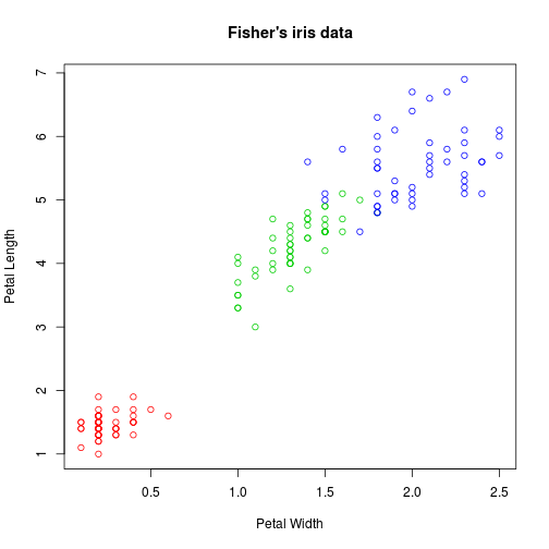
And nicely-formatted tables:
knitr::kable(head(iris))| Sepal.Length | Sepal.Width | Petal.Length | Petal.Width | Species |
|---|---|---|---|---|
| 5.1 | 3.5 | 1.4 | 0.2 | setosa |
| 4.9 | 3.0 | 1.4 | 0.2 | setosa |
| 4.7 | 3.2 | 1.3 | 0.2 | setosa |
| 4.6 | 3.1 | 1.5 | 0.2 | setosa |
| 5.0 | 3.6 | 1.4 | 0.2 | setosa |
| 5.4 | 3.9 | 1.7 | 0.4 | setosa |
To add a new R Markdown posts, simply add a file in the _source directory that follows the convention YYYY-MM-DD-name-of-post.Rmd and includes the necessary front matter. Take a look at the source for this post to get an idea about how it works.
Want a local preview? Run
source('knit.R')
in an R ression to compile the R Markdown files, then run jekyll serve on the command line to preview the site (you will need Jekyll installed for this).